NEW DEMO
Linear Transformations with Animations
Introduction: This is not intended to be a portion of a linear algebra book or standard lecture on Linear Transformations.
Rather it could be used as a "refresher", but more likely it can be used to introduce features in linear algebra to encourage students
to take a course in linear algebra.
This is a demo that connects algebra and geometry. We restrict ourselves to two dimensions so that it is easy to
generate images for the class of functions commonly refereed to as linear transformations or mappings. We will use
some linear algebra, specifically matrices. Matrices for this demo are rectangular-shaped arrays that contain numbers
arranged in rows and columns. (Matrices can also contain variables, symbols, or expressions and are used in a wide variety
STEM, Science, Technology, Engineering & Mathematics, areas.)
This demo can provide students with a better intuitive feel
for the interrelationship between the algebra and the geometry involved, one of the most important foundations of linear algebra.
We provide a brief introduction to related items in simple terms about linear algebra that we will use.
You can use the "Easy Jumps" below to see portions of the tools needed in our simple development which provides animations to
help understand the tools. For some one new to linear transformations we recommend using the contents of the jumps in the order they are listed.
Easy Jumps
Vector
Vector Space
Ordered Pairs
Transformations
Matrices
Matrix Multiplication
Computing Matrix Multiplications
Properties of Matrix Products
Matrix Multiplication is a Linear Transformation
Common Transformations
Translations or Shifts
NOTES
Vector:
In mathematics, a quantity that has both magnitude and direction. Examples of such quantities are velocity and acceleration.
Here is a sample image of a vector in a plane; click this thumbnail
![]()
Vector Space:
A vector space consists of a set of vectors and a set of scalars (numbers) that is closed under (vector) addition and scalar multiplication.
That is, when you multiply any two vectors in a vector space by scalars and add them, the resulting vector is still in the vector space.
In this demo our vector space V is a 2-dimensional Cartesian grid. Click this thumbnail
![]() for an image.
We will only use a portion of the standard Cartesian grid. Click this thumbnail
for an image.
We will only use a portion of the standard Cartesian grid. Click this thumbnail
![]() for an image (we may change the size as needed).
for an image (we may change the size as needed).
Ordered Pairs, alias DOTS:
We will be using dots and connections for images. We will use dots in a portion of a Cartesian grid to construct images like
the thumbnail
![]() and other figures. We will consider the dots as vectors since we will think of them as being connected to the origin which will be a part of the portions of the 2-dimensional
Cartesian grids we use. Click here
and other figures. We will consider the dots as vectors since we will think of them as being connected to the origin which will be a part of the portions of the 2-dimensional
Cartesian grids we use. Click here![]() for a sample of dots with connections.
for a sample of dots with connections.
Transformations:
For this demo, a transformation is 'function' that assigns to each vector in our vector space to a single vector also in our vector space.
A linear transformation T is a function that satisfies two rules: (1) for vectors u and w in our vector space V, the result of T
working on u + w is the same as the sum of T working on u
+ the result of T working on w. (2) for any (real) number k T working on vector k*u is the same as k times the result of T working on u.
Usually these requirements are written as T(u + w) = T(u) + T(w) and T(k*u) = k*T(u). All of our transformations will be linear transformations and their result will appear in
the portion of the 2-dimensional grid that we use for demonstrating that transformation.
Matrices:
As we stated in our introduction to this demo, matrices are rectangular-shaped arrays that contain numbers
arranged in rows and columns. The contents of a matrix are called entries or elements and appear at the intersection of the rows and columns.
The dimensions of a matrix tells its size, the number of rows and columns, in that order. For example
\(
Q =
\begin{bmatrix}
1 & -4& 2 \\
1 & 0 & 2 \\
\end{bmatrix}
\)
is a 2 by 3 matrix and
\(
M =
\begin{bmatrix}
1 & 2 \\
3 & 5 \\
\end{bmatrix}
\)
is a 2 by 2 matrix. Often the size of matrix is written 2 x 3 and 2 x 2, respectively for our examples. In fact, most of the time we will be using 2 x 2 matrices and a single row matrix (1 x n) containing
all the x-co-ordinates and another row matrix for all the y-co-ordinates of the dots.
What are matrices used for in math?
A lot of things, but we will use them in transformations, taking any point in our 2-D vector space and moving it somewhere else.
Matrices are a compact way of talking about and working with a linear transformations.
Matrix Multiplication:
We can multiply matrices, but there are restrictions.
Matrix multiplication is an operation in mathematics that produces a matrix from two matrices.
To perform matrix multiplication, the number of columns in the first matrix must be equal to the number of rows in the second matrix.
The resulting matrix, known as the matrix product, has the number of rows of the first and the number of columns of the second matrix.
The product of matrices A and B is denoted as AB or labeled a new name like C = AB.
An example using our matrices Q and M: the matrix product MQ (a 2 x 2 times a 2 x 3) is valid and the result is a 2 x 3 matrix, but the product QM is NOT valid.
For an image of general matrix multiplication click this thumbnail
![]() .
.
Computing Matrix Multiplications: We use an operation called row-by-column product and sometimes called a dot product of a row and column. The dot product is an algebraic operation that takes two equal-length sequences of numbers and computes the sum of corresponding entries. This computation has the form \[ \begin{bmatrix}a_1 & a_2 & \cdots & a_n \end{bmatrix} . \begin{bmatrix}b_1 \\ b_2 \\ \vdots \\ b_n \end{bmatrix} = (a_1*b_1) + (a_2*b_2) + \cdots + (a_n*b_n) \] where both the row and column have n entries. Note that the result of a dot product is a single number. Check the following example of a dot product. \[ \begin{bmatrix}-2 & 0 & 1 & 2\end{bmatrix} . \begin{bmatrix}1 \\ 1 \\ 3 \\ 2 \end{bmatrix} =11 \] Next we show the product of two matrices \(A = \begin{bmatrix}3 & 4 & 2\\-1 & 1 &\ 0\ \end{bmatrix}\) and \(B = \begin{bmatrix}1 & 0 & -1\\2 & 1 & 1\\ 1 & -1 & 3\\ \end{bmatrix}\) by using dot products of rows of A by columns of B.
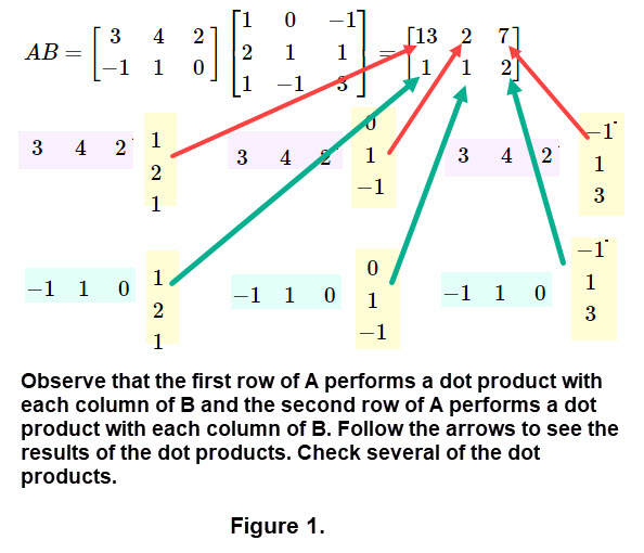
You can copy the matrices if you want to and figure the values of the dot products. (To check, look at a NOTES at the end of this demo; don't cheat.)
Properties of Matrix Products: Let A, B, and C be matrices, x vector, and r be a scalar. Then \[A(B + C) = AB + AC \text{ and } A(rx) = rAx\] These properties are called distributive rules for matrix multiplication over matrix addition. The verification of these expressions uses the technique of matrix multiplication as discussed above. (This assumes that the sizes of the matrices and vector are valid for multiplication.)
Matrix Multiplication is a Linear Transformation: Using the properties of matrix multiplication (immediately above) verifies that matrix multiplication satisfies the rules to be a linear transformation. We will use this in a variety of applications that transform objects like a set of dots that are a geometric shape, graphs of functions, or general plane curves. Here is a list of applications for objects in the plane that appear in many introductory linear algebra courses:
- Moving (rotating, reflecting, translating)
- Resizing (contracting, expanding)
- Changing the Shape (shearing)
Here we explain how to use a matrix to form a linear transformation and compute the result. Since our vector space is 2-dimensional the matrix we use will be 2 by 2 (in most cases); let \( M = \begin{bmatrix}a & b\\ c & d \\ \end{bmatrix} \). The image that is to be transformed will consist of a set of DOTS, ordered pairs (x, y). We construct a matrix from the dots as follows: we use the x-co-ordinates for a first row and the y-co-ordinates for the second row like (we are assuming there are n ordered pairs) \[\begin{bmatrix}x_1& x_2 & x_3 & \cdots & x_n\\ y_1 & y_2 & y_3 & \cdots & y_n \\ \end{bmatrix} \] The equation for linear transformation is \[M*\begin{bmatrix}x_1& x_2 & x_3 & \cdots & x_n\\ y_1 & y_2 & y_3 & \cdots & y_n \\ \end{bmatrix} = \text {the matrix product} \] which will be a new set of n ordered pairs. Carefully look at the following examples.
Example 1:
In this example the image will have its ordered pairs in the two row matrix
\(\begin{bmatrix} 0& 4 & 2 & 2 & 0\\ 0 & 2 & 2 & 4 & 0 \\ \end{bmatrix} \).
To see the image click the thumbnail
 .
For the 2 by 2 matrix M we need to select the entries; we chose \( M = \begin{bmatrix}-2 & 0\\ 0 & 2 \\ \end{bmatrix} \).
To see the result of the linear transformation click this thumbnail
.
For the 2 by 2 matrix M we need to select the entries; we chose \( M = \begin{bmatrix}-2 & 0\\ 0 & 2 \\ \end{bmatrix} \).
To see the result of the linear transformation click this thumbnail
 .
You can see other linear transformations of the original image by clicking here.
Example 1 with buttons.
.
You can see other linear transformations of the original image by clicking here.
Example 1 with buttons.
NOTE: to display matrices in examples we will use a form like [-2, 0\ \ 0, 2] for 2 by 2 matrix
and [0, 4, 2, 2, 0 \ \ 0, 2, 2, 4, 0] for the set of x and y co-ordinates of the image.
Assuming you have clicked on "Example 1 with buttons" and used the buttons you saw a portion of the image which is in the following thumbnail (click it).
![]()
Here are some exercises related to Example 1.
- Use the matrix M and the (x, y) matrix \(\begin{bmatrix} 0& 4 & 2 & 2 & 0\\ 0 & 2 & 2 & 4 & 0 \\ \end{bmatrix} \)
to compute the dots (the ends of the line segments) for each of the 3 figures obtained from the original figure.
- Construct a sentence about the way each of the 3 figures were "moved" and the size changed compared to the original figure.
- If another button was available in "Example 1 with buttons" using the matrix \( M = \begin{bmatrix} 1 & 0\\ 0 & 0 \\ \end{bmatrix} \)
describe the corresponding result.
======================================
Common Transformations: Next we have a list of the names of some common transformations and the matrix M which is used to perform the transformation.
- Reflection about the x-axis; \( M = \begin{bmatrix} 1 & 0\\ 0 & -1 \\ \end{bmatrix} \).
- Reflection about the y-axis; \( M = \begin{bmatrix} -1 & 0\\ 0 & 1 \\ \end{bmatrix} \).
- Reflection about the origin; \( M = \begin{bmatrix} -1 & 0\\ 0 & -1 \\ \end{bmatrix} \).
- Expanding or contracting in both the x and y directions by a factor k; \( M = \begin{bmatrix} k & 0\\ 0 & k \\ \end{bmatrix} \).
- A shear in the x-direction keeps the y-co-ordinates fixed and shifts the x-coordinates horizontally; \( M = \begin{bmatrix} 1 & k\\ 0 & 1 \\ \end{bmatrix} \). Computing a transformation of an ordered pair we get, \( M * \begin{bmatrix} x \\ y\\ \end{bmatrix} = \begin{bmatrix} x + ky\\ y\\ \end{bmatrix} \) which illustrates the shift.
- A shear in the y-direction keeps the x-co-ordinates fixed and shifts the y-coordinates vertically; \( M = \begin{bmatrix} 1 & 0\\ k & 1 \\ \end{bmatrix} \). Computing a transformation of an ordered pair we get, \( M * \begin{bmatrix} x \\ y\\ \end{bmatrix} = \begin{bmatrix} x \\ y+kx\\ \end{bmatrix} \) which illustrates the shift.
- Clockwise rotation by an angle \(\theta \) about the origin; \( M = \begin{bmatrix} \text{cos(} \theta \text{)} & \text{sin(} \theta \text{)}\\ \text{-sin(} \theta \text{)} & \text{cos} \theta \text{)} \\ \end{bmatrix} \).
- Counterclockwise rotation by an angle \(\theta \) about the origin; \( M = \begin{bmatrix} \text{cos(} \theta \text{)} & \text{-sin(} \theta \text{)}\\ \text{sin(} \theta \text{)} & \text{cos} \theta \text{)} \\ \end{bmatrix} \).
- Any 2 by 2 matrix \( M = \begin{bmatrix}a & b\\ c & d \\ \end{bmatrix} \) can be used to create a linear transformation. In this demo we
want to choose matrix entries that keep images in our vector space
 .
.
Example 2: In this example the image will have its ordered pairs in the two row matrix
\(\begin{bmatrix} 0& 5 & 5 & 4 & 3 & 2 & 1 & 0 & 0\\ 0 & 0 & 1 & 1 & 3 & 1 & 2 & 1 & 0 \\ \end{bmatrix} \).
To see the image click the thumbnail
![]() .
This image is called PEAKS. We have buttons that choose a matrix M to generate a common linear transformation that appears in the list above.
You will see this information on the activity; click the thumbnail
.
This image is called PEAKS. We have buttons that choose a matrix M to generate a common linear transformation that appears in the list above.
You will see this information on the activity; click the thumbnail
![]() .
Click here for Example 2 with buttons.
.
Click here for Example 2 with buttons.
Assuming you have tried "Example 2 with buttons" here are some exercises related to Example 2. For each button below name the linear transformation used and
construct the matrix M in each case. (You may want to look at the DOTS in the button's image to help your responses.)
- BUTTON 2 _______________________________
- BUTTON 3 _______________________________
- BUTTON 4 _______________________________
- BUTTON 5_______________________________
- BUTTON 6 _______________________________
=================================
Example 3: We will work with linear transformations involving shears. In general, a shear transformation is one in which all points along a given line L remain fixed while other points are shifted parallel to L. Here we consider only shears in the x-direction and in the y-direction as defined in our list of common transformations above. This is seen in a simple way in Figure 2 below.
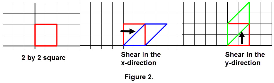
Using the arrows in Figure 2 what is the slope of each of the transformed images? (Hint: look for a right triangle and compute the slope of the hypothesis.) The value of the slope is the number k shown in matrices for shears in the list above.
In this example the image will have its ordered pairs in the two row matrix
\(\begin{bmatrix} -1 & 1 & 1 & 2 & 2 & -2 & -2 & -1 & -1 \\ 0 & 0 & 2 & 2 & 3 & 3 & 2 & 2 & 0\\ \end{bmatrix} \).
This image is called CAPITAL T. We have buttons that choose a matrix M to generate a shear linear transformation which appears in the list above.
You will see this information on the activity; click the thumbnail
![]() Click here for Example 3 with buttons.
Click here for Example 3 with buttons.
Assuming you have tried "Example 3 with buttons" here are some exercises related to Example 3. For each button below name the type of shear transformation used and
construct the matrix M in each case. (You may want to look at the DOTS in the button's image to help your responses. Think about slopes!)
- BUTTON 2 _______________________________
- BUTTON 3 _______________________________
- BUTTON 4 _______________________________
- BUTTON 5_______________________________
=================================
Example 4: We will work with linear transformations involving rotations about the origin. The figures we rotate will be a set of DOTS with connections.
There are several activities.
The first activity involves using a 5-sided figure to rotate 360 degrees. We illustrate the rotation by showing steps.
Buttons will be used to show the steps of the rotation. We use the same angle for each of the steps. The activity has simple directions and the buttons to be used.
Click this thumbnail;
![]() .
In addition there are two questions to consider.
Click here for Rotation of 5-sided figure..
.
In addition there are two questions to consider.
Click here for Rotation of 5-sided figure..
The second activity involves a rose curve. A rose curve is a constructed on a polar graph; see Figure 3.
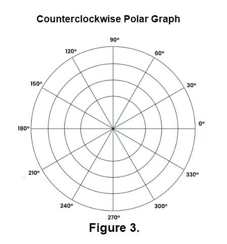
Graphing a polar equation is accomplished in pretty much the same manner as rectangular equations are graphed. Instead of graphing ordered pairs (x, y) you plot polar coordinates (r, \(\theta\)) where r is the value of a polar function evaluated at an angle \(\theta\). The functions in this case are trigonometric expressions.
A rose curve is a graph that is produced from a polar equation in the form of \(r = A*sin(k\theta) \) or \(r = A*cos(k\theta)\), for A not equal to 0 and k is an integer > 1. They are called rose curves because the loops that are formed resemble petals. The number of petals that are present will depend on the value of k. The value of A will determine the length of the petals.
There are a wide variety of rose curves. If k is an even integer, then the rose will have 2k petals. If k is an odd integer, then the rose will have k petals. Examples appear in Figure 4. We chose A = 3 so that the images appear a nice size in our vector space.

Buttons will be used to show a few steps of a rotation for the rose curve. We use the same angle for each of the steps.
The activity has simple directions, in addition there is a question to consider.
Click here for Rotation of a rose curve.
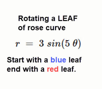
If you look at Figure 4 notice the symmetry of the rose curves. If choose the angle of rotation carefully you can perform a rotation that makes things look like you made a 360 degree rotation in just a few steps. Next we have gif file that starts with a single "leaf" of the rose curve generated by using \(\text{r =3}*sin(5*\theta)\). We start with a blue leaf and rotate 360 degrees that ends with the change to a red leaf. Click here Rotation of a rose curve leaf to see the animation. If you carefully count the leaf displays you can determine the rotation angle.
Another way to look at a rose curve is to see it traced as the (x, y) points are connected on the screen. For an example
click on Trace out a rose curve.
You can do this yourself at Animate a rose curve in GEOBRA .
(Have fun: experiment.)
===============================
Translations or Shifts:
We have investigated general transformations that we listed previously:
rotating, reflecting, contracting, expanding, shearing, and rotations. We need to discuss translations or shifts which
"carry" an image without distortion beyond where it used to be to a new place in our vector space.
Click the following thumbnail for an example:
![]() .
Unfortunately translations cannot be expressed using a transformation matrix that is 2 by 2. In order to perform a translation using matrix multiplication
we need to introduce the notion of homogeneous coordinates which uses a 3 by 3 matrix. This is relatively easy to do using several expiation steps..
.
Unfortunately translations cannot be expressed using a transformation matrix that is 2 by 2. In order to perform a translation using matrix multiplication
we need to introduce the notion of homogeneous coordinates which uses a 3 by 3 matrix. This is relatively easy to do using several expiation steps..
- The translation of a point, vector, or object defined by a set of points in our vector space, is performed by adding the same quantity \(\triangle x\) to each x-coordinate and the same quantity \(\triangle y\) to each y-coordinate. The quantities \(\triangle x\) and \(\triangle y\) are NOT required to be equal in magnitude. We illustrate this in Figure 5 for a point in our vector space, where the coordinates of the translated point are shown.
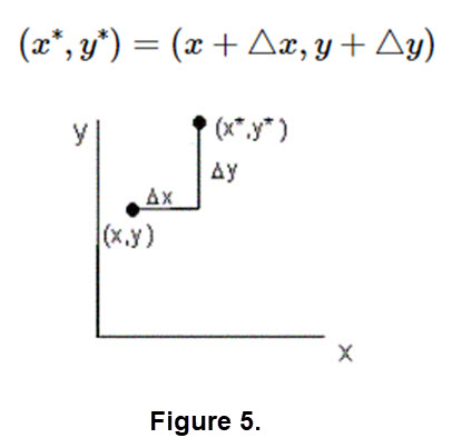
- A point \( (x, y) \) in our vector space is written in the form \(\begin{bmatrix}x \\y \\ \end{bmatrix}\) when we multiply a 2 by 2 matrix \(M = \begin{bmatrix} a & b\\ c & d\\ \end{bmatrix}\). To use homogenous coordinates we use the 3 by 1 matrix \(\begin{bmatrix}x \\y \\ 1\\ \end{bmatrix}\). In a similar way we modify the 2 by 2 matrix M to the form \(M = \begin{bmatrix} a & b & 0\\ c & d & 0\\0& 0 & 1\\ \end{bmatrix}\).
- A translation can be performed by matrix multiplication on data expressed in homogeneous coordinates using a 3 by 3 matrix \(M = \begin{bmatrix} 1 & 0 & \triangle x\\ 0 &1 & \triangle y \\0 & 0 & 1\\ \end{bmatrix}\). Let's call this matrix M the translation matrix.
- Let's do the matrix multiplication with \(M * \begin{bmatrix}x \\y \\ 1\\ \end{bmatrix} = \begin{bmatrix} 1 & 0 & \triangle x\\ 0 &1 & \triangle y \\0 & 0 & 1\\ \end{bmatrix} * \begin{bmatrix}x \\y \\ 1\\ \end{bmatrix} = \begin{bmatrix} x + \triangle x\\ y + \triangle y \\ 1\\ \end{bmatrix} \). The result is in homogeneous form and is like the result in Figure 5.
Example 5: We can show the translation step-by- step that gives you a feel for the power of using the homogeneous coordinates. Each step uses a different transition matrix to make the images from the original image to the target of the transition. Click either (or both) of the following translations: TRANSLATION of a Triangle TRANSLATION of a Rose Curve.
Here is an another example of a translation that uses different translation matrices. Just follow the directions that appear on the image when that you click here TRANSLATION of a SAIL. For a hint to the question in the image see Figure 5.
Example 6: Previously we made rotations about the origin. Here we will provide an example of a rotation about a dot in a figure.
Click the thumbnail
![]() to see the simple figure we will use.
to see the simple figure we will use.
Unfortunately to rotate about a dot that is not the origin the matrix \( M = \begin{bmatrix} \text{cos(} \theta \text{)} & \text{sin(} \theta \text{)}\\ \text{-sin(} \theta \text{)} & \text{cos} \theta \text{)} \\ \end{bmatrix} \) will not do the job. But we have a "tool" that will help us perform a rotation in this case. Here is an activity to illustrate the procedure. Click on Rotation about a DOT. Follow the directions on the screen and answer the question included. Write the type of "move" for the buttons listed below and what angle was used..
- FIRST _______________________________
- SECOND _______________________________
- THIRD _______________________________
- What angle was used in the rotation? ________________
NOTES:
- REVIEW: In most introductory linear algebra courses, prominent applications of transformations
or mappings are moving (rotating, reflecting, translating), re sizing (contracting, expanding),
changing the shape (shearing, projecting) objects in the plane. A typical problem in such courses
is to write the matrix of a transformation that changes points in such prescribed ways.
While one can easily visualize the effect of such a transformation on particular points
or on easily described objects like lines or rectangles, the effect on more complicated
objects like graphs of functions or general plane curves is more difficult to visualize.
The goal of this demo is to help students more easily visualize such transformations on a wide class
of plane objects. Furthermore, use of this demo provide students with a better intuitive feel for the interrelationship between
the algebra and the geometry involved, one of the most important foundations of linear algebra.
- Solutions of the optional quiz on matrix multiplications; EF is not valid since E is 2 by 2 and F is 3 by 3, FG missing values 6 & 38, EG missing values 4 & 22.
-
Example 1 types of transform solutions: The dots for the three figures are as follows.
\( \begin{bmatrix} -2 & 0\\ 0 & 2\\ \end{bmatrix} * \begin{bmatrix} 0& 4 & 2 & 2 & 0\\ 0 & 2 & 2 & 4 & 0 \\ \end{bmatrix} = \begin{bmatrix} 0& -8 & -4 & -4 & 0\\ 0 & 4 & 4 & 8 & 0 \\ \end{bmatrix}\)
\( \begin{bmatrix} 1 & 0\\ 0 & -2\\ \end{bmatrix} * \begin{bmatrix} 0& 4 & 2 & 2 & 0\\ 0 & 2 & 2 & 4 & 0 \\ \end{bmatrix} = \begin{bmatrix} 0& -4 & -2 & -2 & 0\\ 0 & -4 & -4 & -8 & 0 \\ \end{bmatrix}\)
\( \begin{bmatrix} -1/2 & 0\\ 0 & -1/2\\ \end{bmatrix} * \begin{bmatrix} 0& 4 & 2 & 2 & 0\\ 0 & 2 & 2 & 4 & 0 \\ \end{bmatrix} = \begin{bmatrix} 0& -2 & -1 & -1 & 0\\ 0 & -1 & -1 & -2 & 0 \\ \end{bmatrix}\)
Using \( \begin{bmatrix} -2 & 0\\ 0 & 2\\ \end{bmatrix}\) the object is reflected about the y-axis and the size is doubled.
Using\( \begin{bmatrix} 1 & 0\\ 0 & -2\\ \end{bmatrix}\) the object is reflected about x-axis and the y-coordinates are doubled.
Using \( \begin{bmatrix} -1/2 & 0\\ 0 & -1/2\\ \end{bmatrix}\) the object is reflected about the origin and sized was halved.
If \( M = \begin{bmatrix} 1 & 0 \\ 0 & 0 \\ \end{bmatrix}\) the result is a straight line since all the y-coordinates are zero. - Example 2 transform solutions: You were asked to determine the name for each transformation and construct the corresponding matrix M.
We list them by the color of button.
BLUE: contraction (very small), \( M = \begin{bmatrix} 1/4 & 0 \\ 0 & 1/4 \\ \end{bmatrix}\)
GREEN: reflection about the y-axis, \( M = \begin{bmatrix} -1 & 0 \\ 0 & 1 \\ \end{bmatrix}\)
BLACK: reflection about he origin, \( M = \begin{bmatrix} -1 & 0 \\ 0 & -1 \\ \end{bmatrix}\)
AQUA: reflection about the x-axis, \( M = \begin{bmatrix} 1 & 0 \\ 0 & -1 \\ \end{bmatrix}\)
MAGENTA: expanding (doubling in this case), \( M = \begin{bmatrix} 2 & 0 \\ 0 & 2 \\ \end{bmatrix}\)
- Example 3 shear solutions: Name the type of shear and construct he corresponding matrix M. We list them by the color of the button.
BLUE: shear in the x-direction left, \( M = \begin{bmatrix} 1 & -1 \\ 0 & 1 \\ \end{bmatrix}\)
GREEN: shear in the y-direction, \( M = \begin{bmatrix} 1 & 0 \\ 2 & 1 \\ \end{bmatrix}\)
BLACK: shear in the x-direction right, \( M = \begin{bmatrix} 1 & 3 \\ 0 & 1 \\ \end{bmatrix}\)
MAGENTA: shear in the x-direction and doubled, \( M = \begin{bmatrix} 2 & 2\\ 0 & 2 \\ \end{bmatrix}\)
- Example 4 rotation solutions:
Rotating a 5-sided figure(activity) solution: Rotation angle is 45 degrees.
Rotation of a rose curve (activity solution): Rotation angle is 30 degrees.
- Example 5 translation solutions:
Translation of a rose curve (activity) solution: The origin was translated to point (-6, 4).
Translation of a SAIL (activity) solution: The Homogeneous Matrix for the green sail is \( M = \begin{bmatrix} 1 & 0 & 5 \\ 0 & 1 & -6 \\ 0 & 0 &1 \\ \end{bmatrix}\). - Example 6 rotation not about the origin solution:
Rotating around dot (5, 4): First is a translation of (5, 4) to the origin. Second is a rotation at the origin. Third is a translation of the origin back to (5, 4).
The angle used was 45 degrees for the rotation at the origin.
- There are quite a few places on the internet that describe polar graphs, rose curves, and display a variety of rose curves. Here are several
interesting sources:
Plane Curves
Polar Graphs
How to Read a Polar Graph
More information on linear transformations at a higher level
- A further look a homogeneous coordinates than just translations: click here More about homogeneous coordinates.
==============================