Demos with Positive Impact

NEW DEMO

Polynomials, Rationals, and Reciprocals Gallery

Lets take a look at the variety of functions in this gallery. Each of the functions involve polynomials. The focus here is the graphing of such functions which contain coefficients that can be varied and hence the graphs change as the value of the coefficients change. We do not solve any equations to obtain roots or solutions. At times the graphs are smooth and continuous, but other expressions have graphs which are piecewise or involve asymptotes. Some brief information on the gallery functions follows.

You can use the "Easy Jumps" below to move to descriptions of the function categories that are in this gallery and other features of this demo.

Easy Jumps
Polynomials
Constant function
Linear Polynomials
Quadratic Polynomials
Cubic Polynomials
Operations involving Linear Polynomials
Radicals
Power Function
Reciprocal Functions
The Gallery
Notes
Sources

Polynomials: For this demo mathematical polynomials are expressions consisting of a "single" variable and real coefficients, that involves only the operations of addition, subtraction, multiplication, and positive-integer powers of variables. Polynomials appear in many areas of mathematics and science. For example, they are used to form polynomial equations, which appear in a wide range of problems, from elementary word problems to complicated scientific problems; they are used to define polynomial functions, which appear in settings ranging from basic chemistry and physics to economics and social science; and they are used in calculus and numerical analysis to approximate other functions. (There are trigonometric polynomials which are linear combinations of functions sin(nx) and cos(nx) with n taking on the values of one or more natural numbers. The coefficients are usually real numbers.) Portions of this paragraph appeared in Features and uses of polynomials.

" Determining the roots of polynomials, or solving algebraic equations, is among the oldest problems in mathematics. However, the elegant and practical notation we use today only developed beginning in the 15th century. Before that, equations were written out in words." For more information on the history and the development of polynomial notation click here Polynomial history.

The general form of a polynomial is \[\large p(x)= a_{n}x^{n}+a_{n-1}x^{n-1}+\dots + a_{2}x^{2}+a_{1}x+a_{0}\] The degree of a polynomial is the largest exponent in the expression. This gallery shows polynomials of degree 0 through 3.

Constant Function: Here the graph displays a horizontal line that acts like an elevator. Rather "boring"!

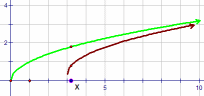
Linear Polynomials: Polynomials of degree 1, linear functions, are one of the most important functions in mathematics. For simple examples using linear functions click this thumbnail (Figure 1). Both examples connect dots. For more information on connecting dots with polynomials click Connect dots; alias, interpolate or Regular polygons.

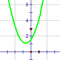
Quadratic Polynomials: Polynomials of degree 2, quadratic functions, also called parabolas, play an important role in a wide variety of applications. "Parabolas can be seen in nature or in manmade items. From the paths of thrown baseballs, to satellite dishes, to fountains, this geometric shape is prevalent, and even functions to help focus light and radio waves." For more detail click on Parabolas in real life. If you follow golf on television you might have seen the path in color when the ball is hit. Two devises like Trackman and Toptracer follow parabolic path. See some more information in this real world application in Selected Resources below the function gallery.

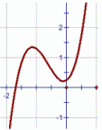
Cubic Polynomials: Polynomials of degree 3 are cubic functions. The geometry here is quite different than that in parabolas. A cubic function with real coefficients has either one or three real roots (which may not be distinct); that is, the graph interjects the horizontal axis in this manner. For more in formation about the graphics click on Graphical features of cubic's. Cubic equations have applications in physics, engineering, and economics, as well as in chemistry to describe the behavior of certain chemical reactions. Both quadratics and cubic are used in computer graphics to create visual effects and in optimization problems to find the maximum or minimum of a function. The curves used in many printing fonts, and in most drawing and graphics programs (like Adobe Illustrator, Power point, etc.), are cubic Bézier curves. Cubic Bézier curves are defined by four control points that mathematically describe the curve: a starting point, an ending point, and two control points. A particular use of this set of cubic curves is to connect dots; click the thumbnail (Figure 2). Note the smooth connecting of the dots; there are no sharp points compared to Figure 1 above.

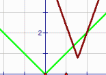
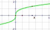
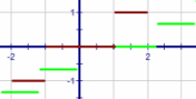
Function Operations involving Linear Polynomials: The inclusion of an absolute value involving the domain values results in a graph of V figure. As the value of the coefficients change so does the "positioning" of the vertex of the V. The inclusion of a step function changes the geometry of the line into pieces. In mathematics, a step function (also called as staircase function) is defined as a piecewise constant function, that has only a finite number of pieces. In other words, a function on the real numbers can be described as a finite linear combination of horizontal lines on given intervals. It is also called a floor function or greatest integer function. The step function is a discontinuous function. Click this thumbnail to see examples. Click here for More on step functions.

Radicals or Roots: In mathematics, a radical or root function is the opposite of an exponent that is represented with a symbol \(\mathbf{\sqrt{ }}\). The origin of the root symbol \(\mathbf{\sqrt{ }}\) is largely speculative. In 1637 Descartes was the first to unite the German radical sign \(\mathbf{\sqrt{ }}\) with the the horizontal "bar" over the expressions inside the radical symbol \(\mathbf{\sqrt{ }}\) to create the radical symbol in common use today.

In this gallery we consider a square root or a cube root of the simple expression \(\mathbf{x - b}\). That is, \(\mathbf{\sqrt{x-b}}\) or \(\mathbf{\sqrt[2]{x-b}}\) for square root while cube root is \(\mathbf{\sqrt[3]{x-b}}\). The number before the symbol or radical is considered to be an index number or degree. Alternatively we could use a fraction style exponent like \(\mathbf{{(x-b)}^\frac{1}{2}}\) or \(\mathbf{{(x-b)}^\frac{1}{3}}\). The domains play an important role for the figures that are displayed. While polynomial functions are defined for all values of the variables, a rational function is defined only for the values of the variables for which the denominator is not zero. Radicals are used in various real world areas like finance and electrical engineering. For example, the financial industry uses rational exponents to compute interest, depreciation and inflation in areas like home buying. and the field of electrical engineering, the use of radical expressions has to do with determining how much electricity is flowing through circuits. One of the simplest formulas in electrical engineering is for voltage, \(V = \sqrt{PR}\), where P is the power in watts and R is the resistance in the measurement of ohms. Portions of these paragraphs appeared in these sources: What is a radical, Radical symbol, and Real world examples of radicals.

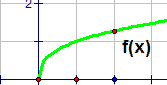
Power Function: In power functions, a fixed value of x is raised to a variable exponent. The exponent or power determines the function's rates of growth or decay. In our demo we chose to use x positive, with x = 2, and varied the exponent b using values in the interval \((-1.25, 5)\). This provides a very simple case of power functions. (The title of power function is used for a different set of functions. Click the following thumbnail to see a familiar set of functions in this other category.)

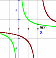
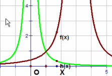
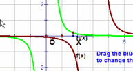
Reciprocal Functions: Reciprocal functions consist of two components: a constant on the numerator and an algebraic expression in the denominator. In this gallery we restrict the denominator to be a simple linear function \((x - b)\) raised to and exponent of 1, 2, or 3. Because \((x - b)\) is in the denominator as x approaches b we will see that asymptotes occur. An asymptote is a line that the curve gets very close to, but never touches. A vertical asymptote of a graph is a vertical line x = b where the graph tends toward positive or negative infinity as the x values approach b. When the function has the form \(\color{red}{y(x) = \frac{a}{(x\, -\, b)^{k} }} \) as in this gallery the horizontal asymptote of the graph is the line y = 0 where the graph approaches the line as the inputs of x increases or decrease without bound. The value of the coefficient a can change how fast the graph converges to an asymptote. (Warning: if your function has the form \(\color{red}{y(x) = \frac{a}{(x\, -\, b)^{k} } + c} \) with c not zero, then the horizontal asymptote of the graph will change. A good source is Reciprocal Functions. )
"One common application is in physics, where they are used to describe phenomena such as simple harmonic motion, electrical circuits, and gravitational forces. In engineering, reciprocal functions are used in fields such as control systems, signal processing, and feedback mechanisms. Additionally, in economics and finance, reciprocal functions can be used to model relationships between variables, such as the inverse relationship between price and demand. Overall, reciprocal functions have a wide range of applications in various scientific, engineering, and economic contexts." Source:Real Life Applications of Reciprocals.

Polynomials, Rationals, and Reciprocals Gallery

The following is a gallery of demos for illustrating selected families of functions. These figures and animations can be used by instructors in a classroom setting or by students to aid in acquiring a visualization background relating to the change of parameters in expressions for functions. Two file formats, gif and MP4, are used and should run on most systems. Originally, see the NOTES below the gallery of animations, the animations were gif files which had no control for a user. The animations are now MP4 files which allow the user to easily control features like stop and go, restart, and change the animation screen size. The controls are similar to those in You Tube. Click this thumbnail to see an example.

Gallery of Animations

\(\text{Constant functions}\) \( \mathbf{ \color{red}{y(x)=c}}\)		Vary c MP4 Animation
\(\text{Linear functions}\) \( \mathbf{ \color{red}{y(x) = mx + b}}\)		Vary m MP4 Animation Vary b MP4 Animation
\(\text{Quadratic functions}\) \(\text{(or parabolas)}\) \( \mathbf{ \color{red}{y(x) = ax^2 + bx +c}}\)		Vary a MP4 Animation Vary b MP4 Animation Vary c MP4 Animation
\(\text{Cubic functions}\) \( \mathbf{ \color{red}{y(x) = ax^3 + bx^2 +cx + d}}\)		Vary a MP4 Animation Vary b MP4 Animation Vary c MP4 Animation Vary d MP4 Animation
\(\text{Absolute value functions}\) \( \mathbf{ \color{red}{y(x) = a\|x - b\| + c}}\)		Vary a MP4 Animation Vary b MP4 Animation Vary c MP4 Animation
\(\text{Greatest integer functions}\) \(\text{(or step functions)}\) \( \mathbf{ \color{red}{y(x) = a[bx - c]}}\)		Vary a MP4 Animation Vary b MP4 Animation Vary c MP4 Animation
\(\text{Square root}\) \( \mathbf{ \color{red}{y(x) = a\sqrt{x - b} + c}}\)		Vary a MP4 Animation Vary b MP4 Animation Vary c MP4 Animation
\(\text{Cube root}\) \( \mathbf{ \color{red}{y(x) = a\sqrt[3]{x - b} + c}}\)		Vary a MP4 Animation Vary b MP4 Animation Vary c MP4 Animation
\(\text{Power functions}\) \( \mathbf{ \color{red}{y(x) = x^{b}}}\), x > 0		Vary b MP4 Animation
\(\text{Reciprocal function}\) \( \mathbf{ \color{red}{y(x) = \frac{a}{x\, -\, b}}}\)		Vary a MP4 Animation Vary b MP4 Animation
\(\text{Reciprocal of x squared function}\) \( \mathbf{ \color{red}{y(x) = \frac{a}{(x\, -\, b)^{2} }} }\)		Vary a MP4 Animation Vary b MP4 Animation
\(\text{Reciprocal of x cubed function}\) \( \mathbf{ \color{red}{y(x) = \frac{a}{(x\, -\, b)^{3} }} }\)		Vary a MP4 Animation Vary b MP4 Animation

Notes

This demo is a modification of a demo in the project Demos with Positive Impact , National Science Foundation's Course, Curriculum, and Laboratory Improvement Program under grant DUE 9952306. managed by David R. Hill and Lila Roberts. The project was based on submitted ideas from instructors. The original demo appeared in 2006.
Special thanks to Deane Arganbright of University of Tennessee at Martin and to Walter Hunter at Montgomery County Community College for their assistance with the development of the Excel files that were used to get this gallery. The book "Mathematical Modeling with Excel", by Erich Neuwrith and Deane Arganbright (Brooks-Cole) provides a rich source of information for developing Excel routines for mathematical instruction.
This gallery was developed by David R. Hill, Temple University.

Selected Resources

The Best of Demos with Positive Impact

An Online Resource for Mathematics Instructors

NEW DEMO

Polynomials, Rationals, and Reciprocals Gallery

Polynomials, Rationals, and Reciprocals Gallery

Gallery of Animations