NEW DEMO

Connect the dots has a variety of meanings. A simple meaning relates to a child's puzzle consisting of a sequence of numbered or alphabetized dots for a picture. The result of following an ordering to connect the dots yields a path from the first dot to the last dot.

Alternatively, connect the dots can mean connect information or ideas to complete a storyline or draw a logical inference to reveal a pattern or formula, or at least to obtain a better understanding of a problem. (To see various meanings or further discussions enter 'connect the dots' to search using your browser.)

Another meaning of connect the dots is interpolation which is related to areas in STEM (Science, Technology, Engineering, and Mathematics). A good description of interpolation is available; click here WIKIPEDIA . A portion is summarized below.

"In the field of numerical analysis interpolation is a type of estimation , a method of constructing (finding) new data points based on the range of a discrete set of known data points. In engineering and science, one often has a number of data points, obtained by sampling or experimentation, which represent the values of a function for a limited number of values of the independent variable. It is often required to interpolate; that is, estimate the value of that function for an intermediate value of the independent variable."

"A closely related problem is the approximation of a complicated function by a simple function. Suppose the formula for some given function is known, but too complicated to evaluate efficiently. A few data points from the original function can be interpolated to produce a simpler function which is still fairly close to the original. The resulting gain in simplicity may outweigh the loss from interpolation error and give better performance in a calculation process."

To start we consider connecting the dots to obtain a picture or a geometric figure from a finite set of dots. Next, we will construct a graph of a path or curve that could lead to a model based on the dot data. However, our primary goal is to present several techniques to compare the geometric behavior of the results. One of the techniques is quite simple, a second technique will be explored in detail, and the third technique will be described with only a few details. Each of these techniques is a form of interpolation but represent only a small part of the descriptions outlined in the Wikipedia summary presented above.

When graphs, curves, or interpolation are involved the adjective "smooth" often appears. There are various interpretations of smooth. For example, from a standard dictionary we find having an even surface; devoid of surface roughness. At times the saying if you trace a curve without picking your pencil off the paper it is smooth is used. In mathematics, smooth curves are often defined more precisely, especially in calculus, numerical analysis, and interpolation.

A curve is smooth if every point has a region where the curve is the graph of a differentiable function. A curve can fail to be smooth if:

• it intersects itself, or
• has a cusp (also called a sharp point).

A curve that is not smooth can be referred to as a path.

For more information click here: Smooth in Calculus .

The following image displays two dot figures which illustrate children's (dot) puzzles. (See Figures 1 and 2.)

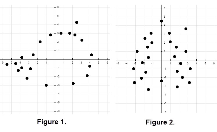
A common part of the puzzle is provided by a numbered sequence of dots to connect or a set of alphabetized dots to connect. We show below a portion of these aids.(See Figures 3 and 4.)

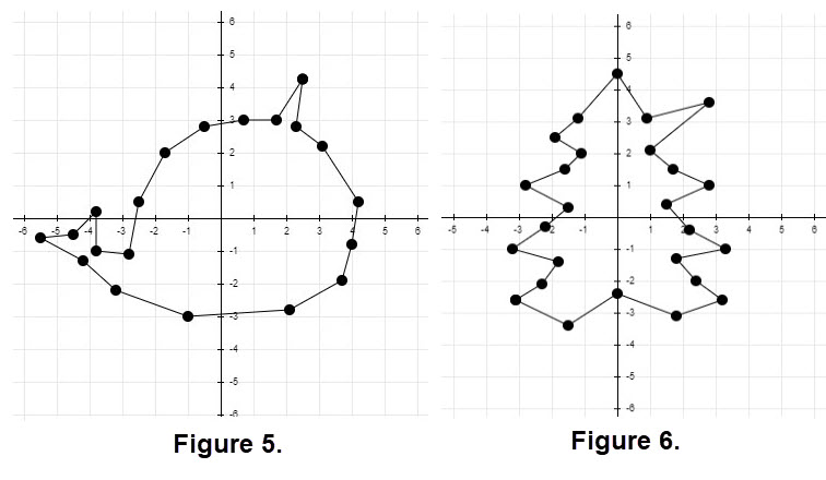
Connecting the dots with straight lines is our first (interpolation) technique. Using straight lines can connect all the dots. It is often the case that there is a "sharp point or cusp" at a dot since the straight lines on either side of the dot may have different slopes. Certainly, this the case for each of our dot puzzles as illustrated in Figures 5 and 6 which are shown next. The connected paths , alias curves, are not smooth.

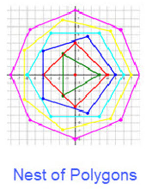
A topic where straight line connections for interpolation is used is in the construction of "regular polygons". The notions of polygons and regular polygons are summarized below.

A polygon is plane figure that has a finite number of sides. The sides or edges of a polygon are made of straight lines segments which are connected end to end to form a closed shape. The point where two line segments meet is called vertex or corner. At a vertex an angle is formed. If the length of all the sides is the same the polygon is called a REGULAR POLYGON. The figure below Nest of Polygons shows a (equilateral) triangle, a square, a pentagon, a hexagon, a heptagon and an octagon. The figure displays these regular polygons in a "nest" and the vertices are represented with a dot. For more information on Regular Polygons click the link Regular Polygons.

Information about java script routines for generating graphs of interpolations in this demo.

All data for the java script in this demo is stored within a routine. We use the term dataset. A dataset is a set of ordered pairs for the dots that will appear on a graph. The ordering of the ordered pairs is imporrtant when using an interpolation method. A detailed summary of the java script routines appears later.

Let's have some fun using straight line interpolation. When we plot the dots on a cartesian grid it may be difficult to see a pattern. Try to guess a name for the dataset image BEFORE you connect the dots. You can do this using a routine by clicking Interpolation via Straight Lines. This routine has 9 datasets of dots. The directions for using this routine are shown below.

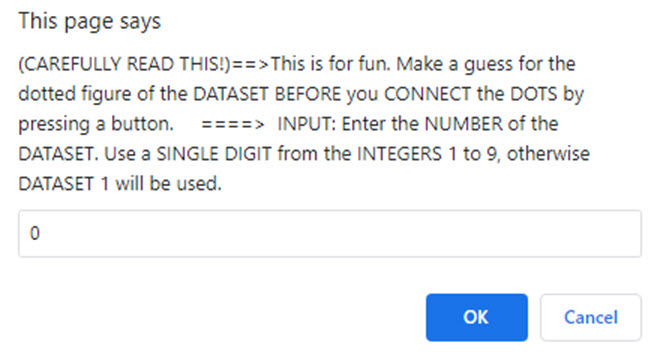
Just click the OK box once you choose an integer from 1 to 9. The dataset of dots will appear. Make a guess, then click the button "Connect via Lines". If you want to try another dataset click the left arrow at the top left of brower's screen. It will take you back so you can click the button "Interpolation via Straight Lines" another time. Experiment! Enjoy!

Looking at the dots in Figure 1 and the straight line connections in Figure 5 a young student may consider using arcs between some of the successive pairs of dots to provide a "roundish" look to certain regions of the dots. Chances are that many arcs still will be joined with a sharp point, but artistically it will be more pleasing. Some of the straight lines used of the left side of the figure seem pleasingly correct.

In our examples we saw that sharp points may be troublesome to connect the dots in an artistically pleasing way. Connecting dots by successive straight lines likely enter and leave a dot with different slopes. If we could develop a connecting technique where the connections enter and leave a dot with the same slope it may provide a better picture quality. This is not a simple problem. One thing we can try is to divide the dots into groups to get a curve (with no sharp points) that goes through each of the dots in the group. With relatively small groups of dots a common interpolation method is to use polynomials.

Polynomials are functions which are the simplest, most used, most important, and provide building blocks for real world models. A polynomial is an expression that consists of variables, coefficients, and constants, which are connected by mathematical operations, such as addition, subtraction, multiplication, and division. We consider only polynomials in a single variable in which the exponents are whole numbers. The general form is \[\Large p(x)= a_{n}x^{n}+a_{n-1}x^{n-1}+\dots + a_{2}x^{2}+a_{1}x+a_{0}\] The degree of a polynomial is the largest exponent in the expression.

Some of the properties of polynomials:

• Polynomials of any degree must have graphs that are smooth and continuous.
• There can be no sharp corners on the graph.
• There can be no breaks in the graph; you should be able to sketch the entire graph without picking up your pencil.
• The graph of a polynomial changes direction at its turning points and the turns are rounded.
• A polynomial function of degree n has at most n - 1 turning points.
• From calculus we know that polynomials are differentiable so we can determine the slope at any point in the domain of the function.

For examples of polynomials just use a browser with "examples of polynomials".

Let's try an example of polynomial interpolation. Suppose we use two groups of adjoined four dots (with a shared middle dot). Then we need two polynomials, one for each group. Each will be a polynomial of degree 3, which has four coefficients. To create such an interpolating polynomial, we need to set up an algebraic expression for each of the four dots using the coordinates of the dots.

For the first group use dots 12, 13, 14, and 15 from Figure 3. The dot 15, which has coordinates (2.1, -2.8), is at the end of the first group (looking from left to right) and will be at the start of our second group of four dots, namely dots 15, 16, 17, and 18. (It is easy to count the dots just use Figure 3.) The coordinates of the first group are respectively \[\large {(x, y): (-4.2, -1.3), (-3.2, -2.2), (-1, -3), (2.1, -2.8)}\]. The coordinates of the second group are respectively \[\large {(x, y): (2.1, -2.8), (3.7, -1.9), (4.0, -0.8), (4.2, 0.5)}\].

Let's use \(\large p_{1}(x)\) for the polynomial of the first group of dots, and \(\large p_{2}(x)\) for the second group of dots. Each of these polynomials will be a smooth graph with \(\large p_{1}(x)\) over interval [-4.2, 2.1] while \(\large p_{2}(x)\) is over interval [2.1, 4.2]. ( It is a coincidence that the intervals have he same length.) We need to check the behavior of the left side and right side at dot 15 to see if there is a sharp point. The computation of the two polynomials in this case can be found by clicking on POLYNOMIAL EQUATIONS. The result of the computation is \[\Large p_{1}(x)= - 0.013783 x^{3} + 0.05184 x^{2} + 0.053112 x - 3.0125 \] \[\Large p_{2}(x)= 1.9361 x^{3} - 17.3728 x^{2} + 51.3006 x - 51.9474\]

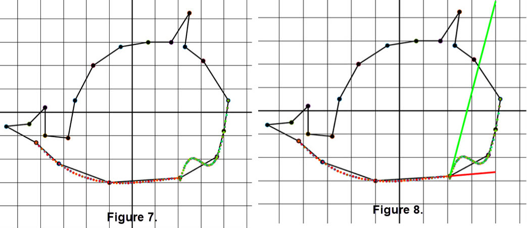
Then, using a bit of calculus we can check the slope at the left of dot 15 and at the right of dot 15 because we have the two polynomials. Differentiate each polynomial and evaluate the derivatives at x = 2.1. At dot 15 at the left the slope is m = 0.0887, while on the right the slope is m = 3.9494. The result is that we have a sharp point at dot 15. See Figure 7 for the graphs of the polynomials and Figure 8 shows the slopes at dot 15. (These figures were enlarged a little to emphasize the polynomials and slopes.)

The experiment with adjacent of two sets of four dots showed that we could "Divide" the set of dots for a figure. The use of polynomial functions may provide a scheme to help "Conquer" the interpolation procedure. We saw that sharp points could happen using sets of four points so maybe we could consider using fewer dots.

Divide to Conquer is a common approach in solving problems. This technique has three phases:

• Divide: Split the problem into smaller sub-problems.
• Conquer: Solve the sub-problems.
• Combine: Combine the sub-problems to solve the whole problem.

For more information on such a procedure look at Divide to Conquer.

There is a technique that divides the dots of a figure so that between successive points we can construct a polynomial of degree 3. (So there are lots of sub-problems.) Each sub-problem needs the two successive dots and a slope at each dot. The technique is called Bézier polynomials which are smooth continous curves between the two dots.. There are different types of Bezier curves which are commonly used in computer-aided geometric design and related fields. We will focus on Cubic Bezier Polynomials which are smooth curves.

BACKGROUND:
A Bézier curve is named after French engineer Pierre Bézier, who used it in the 1960s for designing curves for the bodywork of Renault cars. Pierre Bézier was one of the founders of the fields of solid, geometric and physical modelling as well as in the field of representing curves, especially in computer-aided design, manufacturing systems, and animations. For more information on Pierre Bézier go to Pierre Bézier . For more information on Bézier curves and the under lying mathematics go to Bézier curve .

We want to show how cubic Bézier curves can be manupulated to change shapes and eventually show how the cubic polynomials that support the curves play a role in interpolation possibly without sharp points.

Changing Shape:

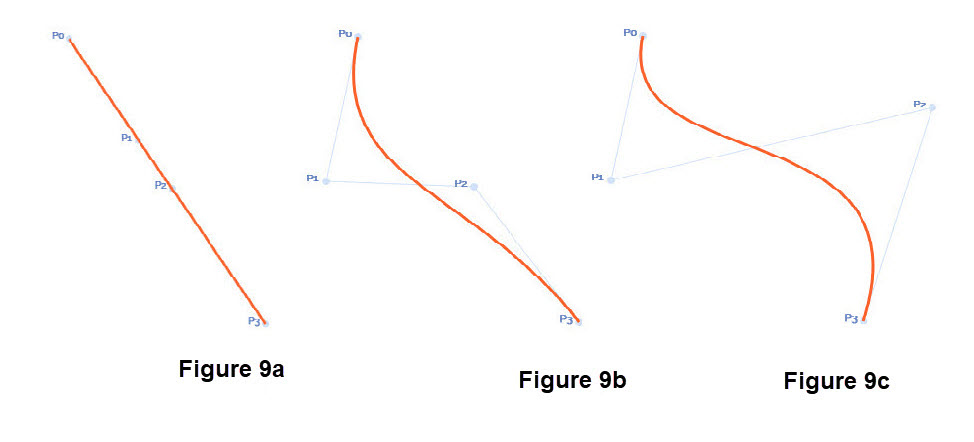
We will keep things simple and provide geometric images regarding the change of the shape for a cubic Bézier curve. This can be illustrated graphically using "two fixed points and two control points which are tied to the fixed points". The line segments that connect a fixed and a control point provide a slope at a fixed point. (Sometimes there is a line connecting the two control points in figures.) From an algebraic point of view we have four constraints on the cubic Bézier polynomial: the curve interpolates the two fixed points and the slopes of the connecting line segments give us two more constraints to compute the four coefficients of the cubic polynomial. Figure 9 shows the geometry of several situations.

COMMENTS on Figure 9.

In Figure 9 the fixed points are \(P_{0}\) and \(P_{3}\) and the control points are \(P_{1}\) and \(P_{2}\).

In Figure 9a we put the control points on the line segment between the fixed points; in this case the equation of the line segment is the cubic Bézier curve.

In Figure 9b we moved control point \(P_{1}\) to the left. The light line segment connecting the \(P_{0}\) to \(P_{1}\) and light line segment connecting the \(P_{3}\) to \(P_{2}\) provide slopes at the two fixed points. The resulting cubic Bézier curve is smooth.

In Figure 9c we moved control point \(P_{2}\) to the right. The result is that we have a change in the slope of the light line segment connecting the \(P_{3}\) to \(P_{2}\) The resulting smooth cubic Bézier curve has changed.

The fixed points are also called the interpolation points. In addition, in many descriptions of codes for picutues of a Bézier curve the terminology control points is applied to the interpolation points. The reason for this is that when trying to model a figure or curve you often want to move the interpolation points to develop a better fit for the model.

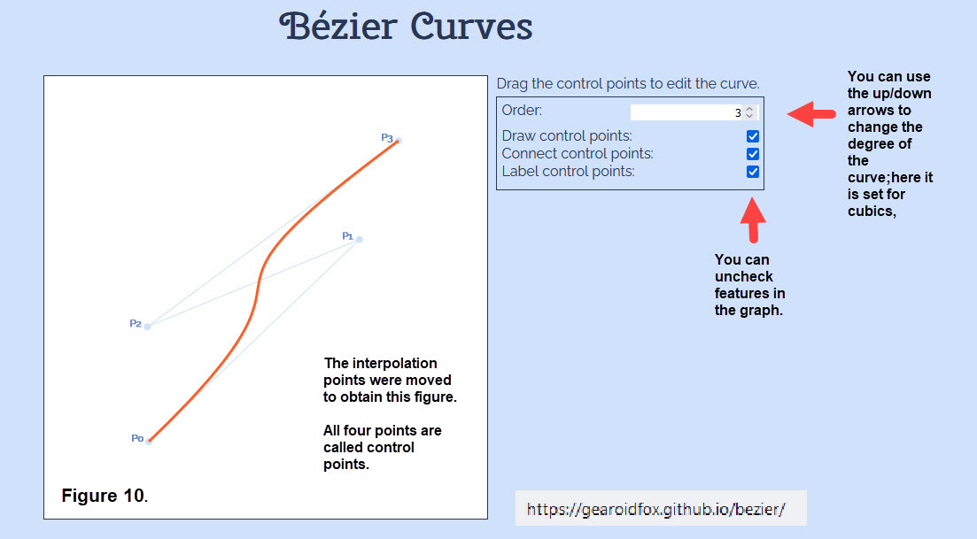
The images in Figure 9 came from using the graphic tool in resource Bézier Curves. Figure 10 shows the main page which is followed by a mathematical description of Bézier curves together with examples and animations. You can "play" with the graphic tool to create various shapes and you can move the interpolation points. This resource really helps to get a feel for cubic Bézier curves. We have annotated feaures available for users of this resource.

"Bézier curves can do a lot of things. You can use them to draw shapes and design patterns, to name one example. They can also be used mathematically, in place of a linear representation of change, shifting gradually and subtly between one keyframe or value and another later on. You might recognize this application in animation programs like Adobe Animate, but the use of Bézier curves goes far beyond the world of art."

"While the artists of the world have certainly taken this concept and skedaddled with it, its mathematical roots make it extraordinarily useful in a number of other professions and disciplines, as well."

"A few other applications for Bézier curves aside from art and design include:"

• "Architecture and construction, such as in the design of superhighways."
• "Industrial design, including the design of toys, furniture, and automobiles."
• "Robotics—Bézier curves can assist in computer-aided locomotion and area-mapping."
• "3D scanning in a biomedical context, where a digital object is created from many 2D cross-sections of the real thing (things like CT scans, to name one example in particular)."

The quoted material is from What Are Bézier Curves in Computer Graphics? which has additional material including figures and information on a range of software that uses Bézier curves.

If you want to experiment with another resource involving cubic Bézier curves consider Try to match a curve. This resource has two fixed points and two control points. Move the control points to match curves that are listed. Another resource is at Build cubic segments. This resource lets you construct multiple segments of a cubic Bézier curve. You can add interpolation points and control points.

Previously

We discussed Bézier curves and polynomals in examples where you needed to make choices for control points (that were not fixed points) in order to provide slopes at the fixed points. When trying to make a model for a particular curve it is important to make choices that render the appropriate shape. Each of the two resources illustrated in Figures 9 and 10 you could experiment and get a feel for the role of the slopes at the fixed points (also the called the interpolation points). If you have tried the resource "Build cubic segments" you could have added segments that had sharp points. Next we want to have (hopefully) no sharp points for Bézier curves built from segments. (There are sharp points that can occur based on the dataset.)

Interpolation using cubic Bézier polynomials depends on the type of the dataset.

Here are items that have a role in various Bézier interpolations.

• We will need to have a dataset of dots/points with x- and y- coordinates and an ordering of the data. These points are the dataset for interpolation; you can't move them,consider them fixed (control) points.
• We may have a dataset like those in Figure 1 that generate a "path", not a curve.
• We may have a dataset that could generate a "path" that crosses itself.
• We may have a dataset that are sorted so that the x-coordinates are ascending.
• We will use a java script code that determines control points so that the Bézier curves will have "no" sharp points between the interpolation points. At the interior interpolation points the slope to the left and that to the right are the same. There will be exceptions; the first and last points will not have control points and there may be places where a slope is infinite and a point is "skipped". This will be discussed later when we explain some of the algorithm in the code.

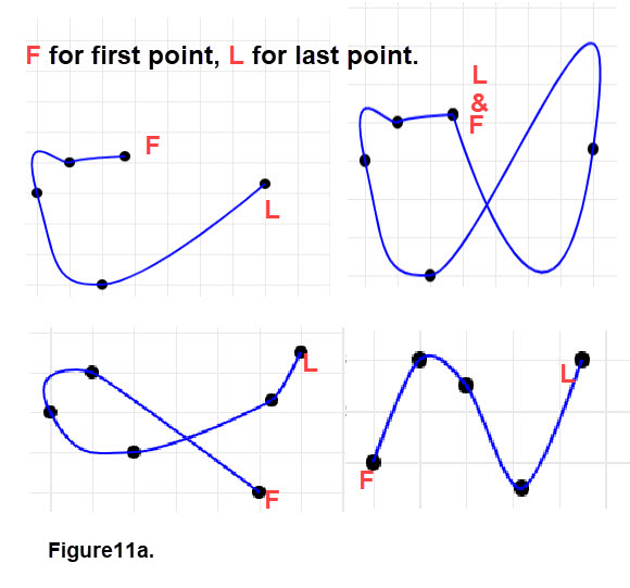
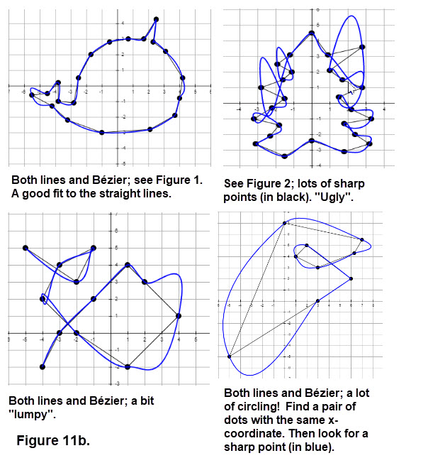
Several examples of paths and cubic Bézier curves are displayed in Figure 11a. Compare the figure with the items in the previous list. Do you see any sharp points? Which figures have paths? Are there any smooth curves?

Interpolation using either straight lines or cubic Bézier curves.

Figure 11b shows other results of cubic Bézier interpolations. Some are quite pleasing and one is definitely "ugly". Look at the notations carefully,

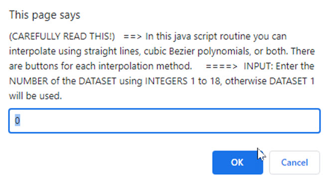
The next java script routine has 18 datasets. Datasets from 1 to 9 are the same as those used for "interpolation using straight lines". The datasets numbered 10 to 18 are a variety that produce other figures. It is highly recommeded that you experiment to see interesting results paths and curves. Look for sharp points. You can do this by clicking Interpolation: Two Methods. The directions for using this routine is shown below. Just click the OK box once you choose an integer from 1 to 18. The dataset of dots will appear. If you want to try another dataset click the left arrow at the top left of brower's screen. It will take you back so you can click the button "Interpolation: Two Methods" another time.

Description of the code used in the java script.

We have pieced together java script codes to produce graphics of cubic Bézier curves. We focus on the following portions:

• the datasets for the interpolation points
• the computation of the control points
• the construction of the Bézier cubic polynomials
• the grid for the graphing

Pieces of code were incorporated from several sources (which are cited in the graphics programs) and we added material of our own.

===> The interpolation points are stored in "datasets" to make it easier for users. (An ordering of the interpolation points is required.) Several different datasets can be selected in our java script programs, but a user could add their own material by editing the java script.

===> Control point computation for the individual members of a data set uses an algorithm by generating one control point to left and another to the right of an interior interpolation point. To see how this is done let's label an interpolation point as curP. We proceed by using another interpolation point preP (which precedes curP) together with one more interpolation point nexP (which follows curP). Now compute the slope from preP to nexP along with the difference in the x-coordinates of nexP and curP. These two quantities are used to obtain a "tweak" in the coordinates of curP which yields one control point. A second control point is determined using a previously computed "tweak" in the coordinates of preP from the preceding step of the algorithm. (Go to the code and look for a "tweak" (dx2, dy2) and another (dx1, dy1). Note that "tweaks" are ordered pairs.) The algorithm basically gives the first and last point with a one sided "tweak" of zero.

===>We use the interpolation points and the control points as information which is sent to a java script function bezierCurveTo to draw the cubic polynomial from the preP to the curP. The control points appear on at the left and right side of curP and the corresponding slopes are the same value.

===>The grid for graphing can be adjusted to provide a variety of horizontal and vertical axes. We have made choices for "grid size" and "distance grid lines" that yield grids which are square and use these square grids in our graphics.

Next we construct an example for data set x = [-5, -3, -1, 2, 4, 4], y = [ 5, 2, 0, -1, 2, 4]. Figure 12a shows the Bézier curve and we illustrate the action of the code steps. Just follow the color of the names and the lines for the 3 interpolation points that would get control points. Figure 12b adds the control points and the slopes on each side of a interpolation point (except for the first and last interpolation point).

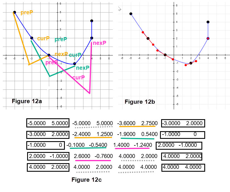
Figure 12c provides numerical data for the computed control points; just coordinate the colors with Figure 12a. The dashed under lines are for control points which do not change anything. The black boxes are the interpolation points.

For a view of the pieces of interpolation for using straight lines and cubic Bézier polynomials click on Step-by-Step which is a slide show that reveals the "behind the scenes" for a set of interpolation points for a more complicated figure.

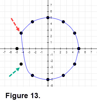
Inspect Figure 13. If the interpolation point at the red arrow is preP and the interpolation at the green arrow is the nexP, what is the slope between these two points? Recall our previous discussion about items computed to "tweak" things to get control points. (Hint: the interpolation points are equispaced around a circle.) This type of behavior occurs for some datasets.

We have shown examples of cubic Bézier interpolations that worked well but at other times there were examples that indicated that this method of interpolation has pitfalls. (See Figures 11a and 11b.) A natural question is, when can we be sure that we eliminate the pitfalls? Of course this is dependent on the dataset of interpolation points. Following is a description of datasets that "behave"!

All of following restrictions on the dataset must be met:

• the x-coordinates are ascending
• the ordered pairs of the dataset are a function; that is, each x-coordinate has exactly one y-coordinate
• the order of the dataset uses the ascending x-coordinates

These restrictions correspond to the behavior of selecting data points from left to right from a curve which is a function. Intuitively, if the spacing between successive x-coordinates is "generous" the resulting curve of cubic Bézier pieces should flow in a nice wave pattern. Continuing, if the selection of ascending x-coordinates is "dense" the resulting curve of cubic Bézier pieces may have lots of close turns, but no sharp points. These two general descriptions are conjectures. To see several examples click on Some figures for ascending datasets.

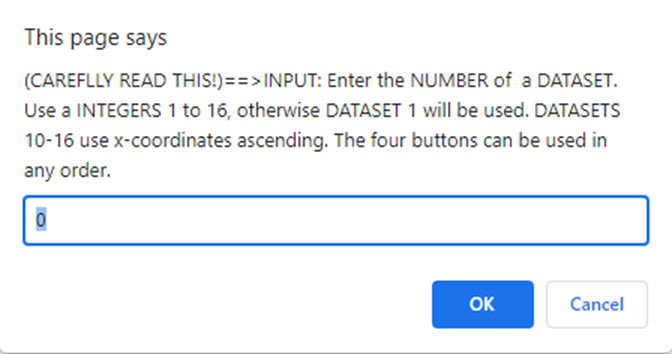
The third java script routine has 16 datasets. Datasets from 1 to 9 include Figure1, some loops, some circlar sets, etc. Datasets 10 to 16 use ascending datasets in which some datasets choose x-coordinates in a psudo random fashion within specified intervals between -14 and 14 with the y-coordinates obtained in a similar fashion. The actual number of points generated also varies. The routine has buttons that permit straight line interpolation, cubic Bézier interpolation, and viewing the control points with finite slopes. The four buttons can be used in any order. Feel free to experiment and display different situations.In particular look at the "red" controls. You can do this by clicking Interpolations and Control Information. The directions for using this routine are shown below. Just click the OK box once you choose an integer from 1 to 16. The dataset of dots will appear. Click the buttons in any order. If you want to try another dataset click the left arrow at the top left of your brower's screen. It will take you back so you can click the button "Interpolations and Control Information" another time.

Our third interpolation technique uses an idea that is like that in cubic Bézier interpolation. This new technique constructs cubic polynomials between successive dots in a dataset , however it uses a different method to compute the cubic polynomials than those used in cubic Bézier interpolation. The name of this interpolation method is Natural Cubic Splines.

Spline Background:
In mathematics, a spline is a 'special function' defined by piecewise polynomials. In interpolation, spline interpolation (there are several types) is often preferred to techniques using polynomials of higher degree. Spline techniques are often discussed in detail in courses in Numerical Analysis. The term spline comes from the flexible spline devices used by shipbuilders and draftsmen to draw smooth shapes. (Adapted from wikipedia.) For additional information go to WIKIPEDIA Splines . More on the history of splines is available by opening the pdf file Spline History.

Dataset restrictions for Natural Cubic Splines are the same as those for elimination of the pitfalls for \( x_1 < x_2 < \dots < x_{n-1} \): 1. The x-coordinates are ascending. 2. The ordered pairs of the dataset are a function; that is, each x-coordinate has exactly one y-coordinate. 3. The order of the dataset uses the ascending x-coordinates.

General Description of Natural Cubic Splines
Natural cubic splines are an interpolation tool that is of interest to many applications. It is a piecewise cubic function that is twice continuously differentiable. For example, suppose we have a dataset which satisfies the three restrictions listed above and the x-coordinates are \(x_0 < x_1 < x_2 < \dots < x_{n-1} < x_n\). We want to construct a cubic piecewise function S(x) where it is made up of the cubic pieces \(s_j(x)\) on the subintervals \( [x_j, x_{j+1}]\) for \(j \,= \,0, 1, 2, \dots , n-1\). This means that S(x) has the following form

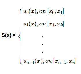
where \[s_j(x) = d_j(x-x_j)^3 + c_j(x - x_j)^2 + b_j (x - x_j) + a_j \; for \; j \,= \,0, 1, 2, \dots , n-1.\]

We require that:

• \(\textbf{S(x)}\) interpolates all the n + 1 points in the dataset.
• \(\textbf{S(x)}\) is continous on the interval \([x_0, x_n]\).
• \(\mathbf{S'(x)}\) is continous on the interval \([x_0, x_n]\).
• \(\mathbf{S''(x)}\) is continous on the interval \([x_0, x_n]\).
• \(\mathbf{S''(x_0) = 0}\) and \(\mathbf{S''(x_n) = 0}\).

The requirements listed above guarantee that S(x) will generate a smooth curve.

To determine the natural spline S(x), which is based on n different cubic polynomials each containing 4 coefficients, we need to solve for a total of 4n unknowns. (Look at the expression of for \(s_j(x) \) ). Using the requirements listed above we have:

==> Interpolation provides n + 1 equations.

==> Continuity of S(x) together with continuity requirements for S'(x) and S''(x) provides 3(n - 1) equations. (Note that continuity applies only to the interior x-coordinates \(x_1 < x_2 < \dots < x_{n-1} \).

==>The final requirement involving the second derivative of S(x) at \( x_0 \) and \(x_{n-1} \) provides 2 more equations.

==> Hence we have a system of 4n unknowns and 4n equations to solve. This is done by solving the approriate linear system of equations which uses matrices.

This is mathematics that is different from the cubic Bézier interpolation. Solving such systems of equations by hand is NOT recommended. Clik here for an Example of a Natural Cubic Spline. which illustrates a simple problem.

As we did with the Bézier interpolation we want to look at some examples but, now using Natural Cubic Splines. In many experiments you try an example based on a situation you can easily check. So let's take the function \(\large f(x) = \frac{x}{0.25 + x^2}\) which is a serpentine curve. Next choose the ascending x-corrdinates \([-2, -1, -0.5, -0.25, 0, 0.25, 0.5, 1, 2]\) from interval [-2, 2] and compute the corresponding y-coordinates to get \([-0.47059, -0.8, -1, -0.8, 0, 0.8, 1, 0.8, 0.47059]\). So we have a dataset which to compute the corresponding interpolation natural cubic spline approximation. Since it makes sense to compare the corresponding cubic Bézier interpolation we display four items in Figure 14. The function graph used x-coordinates at a spacing of 0.01 from -2 to 2 and connected ordered pairs to obtain the figure.

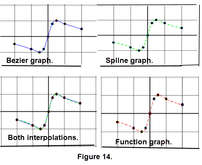
From the graphs in Figure 14 it seems that both the cubic Bézier interpolation and natural spline interpolation performed quite well. However, could you have guessed that? Note that f(x) is a function which has derivatiives of any order and hence has a nice smooth graph. In addition, we chose the dataset so it contained points near places where the smooth graphic's curve significantly changed and where it crossed the x-axis. So you could say we "rigged" things to get good results.

Let's consider another situation. You have a large material that is to be part of a sail. You layed out the material and anchored it so you could draw a curve on it. In addition, you can lay a Cartesian grid on the materal to choose ordered pairs for a dataset. Next, you use your computer to generate an interpolation of the members of the dataset and sketch an image of the resulting curve. With a little more effort you could compare the cubic Bézier interpolation and the natural spline interpolation to determine which image to program into your auto-cutting machine. To see an "idealized" picture of this situation look at Figure 15.

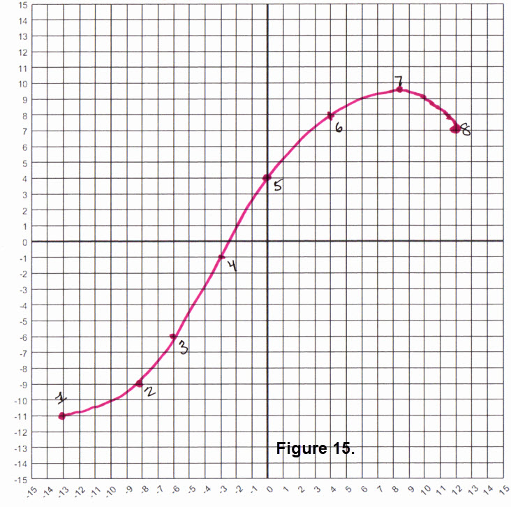
The dataset of 8 estimated ordered pairs is \((-13, -11), (-8, -9), (-6, -6), (-3, -1), (0, 4), (4, 8), (8.5, 9.5), 12, 7)\). Figure 16 contains the intrpolation curves; Bezier in blue and natrual cubic spline in green.

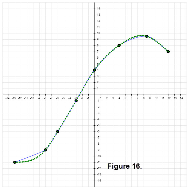
Which interpolation would you choose as the better curve? The impression you get from the second dot may be that there is a sharp point under the dot. But cubic Bézier interpolation creates a smooth curve. If we remove the second dot you would see a small bend in the curve. For a quick look at this click on No sharp point there.

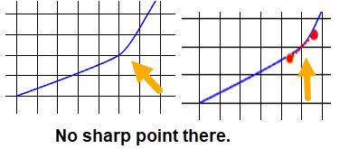
Next consider a zig-zag arrangement of 13 ordered pairs along the x-axis. Figure 17 shows the Bézier interpolation (in blue) and the natural spline interpolation (in green). Which would you choose as the better smooth curve in this case?

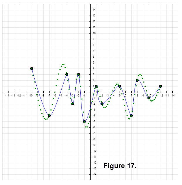
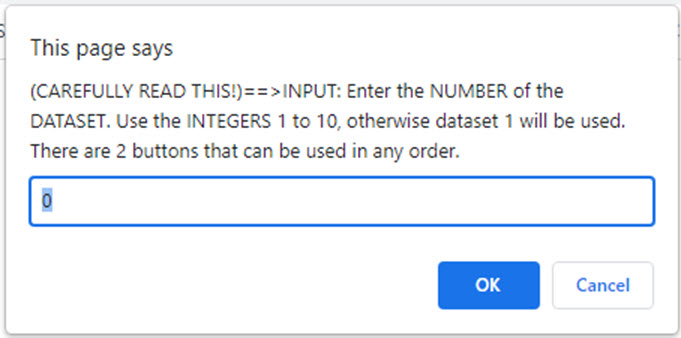
Figures 16 and 17 illustrate the way interpolations for Bézier and natural splines can vary depending upon the dataset. The fourth java script routine has 10 datasets. Explore using this routine; you might want to make guesses for the type of dataset. For instance datasets possibly taken from an old wooden roller coasters, a skate board glide, an alphabet letter, a diagram of a flower pot, or just a random set of ascending x-coordinates. You may want to choose which would be the better smooth curve in the graph that is generated. You can use this routine by clicking Bézier and natural splines. The routine has only two buttons, cubic Bézier interpolation and natural spline interpolation. The buttons can be used in any order. The directions for using this routine are shown below. Just click the OK box once you choose an integer from 1 to 10. The dataset of dots will appear. If you want to try another dataset click the left arrow at the top left of your brower's screen. It will take you back so you can click the "Bézier and natural splines" another time.

SUMMARY:

We have discussed three interpolation schemes and provided examples. The four java script routines let you explore a variety of datasets using the interpolation schemes. Some of the graphs generated showed good interpolation results while others were hard to interpret but did provide situations which indicated pitfalls in some schemes. Comparing the interpolations of Bézier and natural splines for different datasets was not simple and illustrated the influence of datasets. The Bézier and natural splines play important roles in many instances for design and computational situations. In fact, both Bézier and different types of splines (especially B-splines) can be used together. Using your browser, you can find a wide range of uses and information about the interaction of Bézier and splines. It is beyond the scope of this demo to discuss such topics in detail. For a brief discussion of splines and B-splines (basis spline) click on What is the difference Between Natural Cubic Splines, Bézier Splines and B-splines or click on Difference between Splines, B-splines and Bézier Curves.

An Optional Example:

To see the optional example, which is based on a profile curve from an important character, click on Character Profile..

Similar MATLAB Files:

We have two MATLAB files that are similar to the java script files you had access to above. Click here for description: Description of MATLAB files. For a look at the type of output from either MATLAB file click here .
The two MATLAB files can be download/copied by clicking on the two items below:
FIRST MATLAB FILE
SECOND MATLAB FILE.
You can also contact us for these files.