Objective: This demo builds a toolbox of teaching aids to illustrate various aspects of volume calculations using the method of shells. Several props are suggested to demonstrate the geometric ideas of "shells" and the notion of "nesting" shells to obtain an approximation of the volumes of solids of revolution. A collection of animations is included which can be run on a number of platforms, along with some interactive tools using Geogebra.
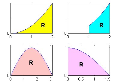
Assumptions: For this demo, we focus on regions bounded by the graph of a continuous function y = f(x) on the interval [a,b], the vertical lines x = a and x = b (where the values of a and b are defined for each example). For the illustrations we also require that f(x) is nonnegative over [a,b]. Several regions of this type are shown in Figure 1.
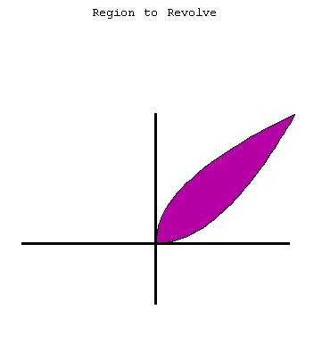
In addition to regions of the type illustrated in Figure 1, we consider regions that are bounded between the graphs of two functions y = f(x) and y = g(x) such as the shaded region in Figure 2.
The region is revolved about the y-axis to generate a solid of revolution, as shown in Figure 3. By dragging the slider below we see how the solid is generated generated by revolving the region about the y-axis.
Strategy: The method of shells is particularly useful when a region is revolved about a vertical axis. The strategy for developing the integral for computing the volume of the resulting solid is based on approximating the volume by filling the solid with cylindrical shells. To illustrate this and motivate the approximation scheme, there are some props that can be useful.
Central to the development of the method of shells is the idea of nesting or layering of the approximating elements. The idea of nesting can be introduced using the layers of an onion (Figure 4).
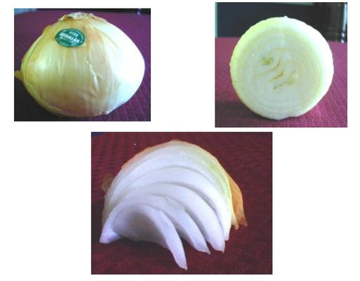
The onion is made up of layers so the volume of the onion could be approximated if we could add up the volume of each of the layers.
Another useful prop to illustrate this idea is a set of Matroyska dolls. In Figure 5, we see that the hollow dolls of varying sizes nest together compactly.
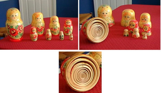
Once students understand how the approximating elements will fit together, we need to show what kind of approximating element we will use and how to compute its volume.
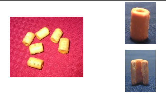
The snack crackers, Combos (Figure 6), are excellent props to illustrate the cylindrical shells. Sharing these crackers with students is a fun way to help them develop the visualization skills that can help give meaning to the approximation scheme. It is easy to see that the cylinder has an inner radius and an outer radius.
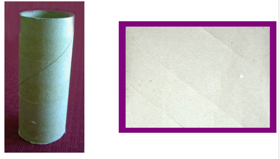
To motivate how to compute the volume of a cylindrical shell, a paper towel roll or toilet paper roll is handy (Figure 7). An intuitive approach to approximating the volume can be obtained by cutting the roll open and flattening it to get a rectangular solid that is very thin. If the rectangular solid is thin enough, the inner and outer radii are close to being equal.
If we analyze the volume of a rectangular solid illustrated in Figure 8, we see that the volume of the solid is equal to the area of the rectangular face multiplied by the thickness. This suggests that we can approximate the volume of a cylindrical shell by thinking of it as a rectangular solid. The length of the face is equal to the circumference of the circle and width equal to the height of the face. If the rectangular solid in Figure 8 approximates the cylindrical shell, the volume V is
$$\text{V}=2 \pi r \times \text{Height} \times \text{Thickness}$$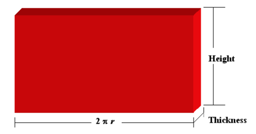
Another way to think about the volume of the cylindrical shell as the volume of a cylinder with height h and a given outer radius less the volume of a smaller cylinder with height h and a given inner radius, as illustrated in Figure 9.
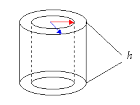
Now we can calculate the volume of the shell. Let rout be the outer radius and rin the inner radius. Then $$\begin{align}V&=\pi r_{out}^{2}h-\pi r_{in}^{2}h \\ &= \pi h(r_{out}^2-r_{in}^2) \\ &=\pi h(r_{out}+r_{in})(r_{out}-r_{in}) \\ &=2\pi h\big(\frac{r_{out}+r_{in}}{2}\big)(r_{out}-r_{in}) \\\end{align}$$
Let $r_{avg}=\Large{\frac{r_{out}+r_{in}}{2}}$. We also recognize that the thickness of the shell is $r_{out}-r_{in}$. So we see that the volume of the shell is $$V = 2 \pi r_{avg}h\times \text{ Thickness}.$$
To see how a shell can be generated as a solid of revolution, think about the region bounded by the graphs of $f(x) = \sqrt{x}$ and $g(x) = x^2$ that we saw earlier in Figure 2. If we partition the interval from x = 0 to x = 1 into parts and draw a resulting rectangle, then by revolving the rectangle about the y-axis, we see that a shell is generated. In the figure below, drag the slider to see how a partition, approximating rectangle, and approximating shell are generated.

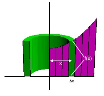
We're now ready to put these ideas into the context of volumes of solids of revolution. In this particular example, the function is $f(x)=x^2+1$ and the region to be revolved about the $y$-axis is the region bounded by the graph of $y = f(x)$, the $y$-axis, the $x$-axis, and the vertical line $x$ = 1.We can think of a shell as being "generated" by a rectangle with height $f(x)$ and width $\Delta x$ . If the graph of $y = f(x)$ is revolved about the y-axis, the average radius of a shell is measured from the axis of revolution, given by $x$. The height of a shell is $f(x)$, and the thickness is $\Delta x$ , shown in Figure 11. For easier visualization, the illustration in Figure 10 shows a half-shell constructed by revolving the rectangle about the $y$-axis.
If we have a region bounded by the graph of $y=f(x)$ and the $x$-axis on the interval $[a,b],$ we set up a partition of the interval $[a,b]$, ${x_0,x_1,x_2, ...,x_{k-1},x_k}$, where the length of each subinterval is $\Delta x$. The volume of the $k^{th}$ shell is $$V_k=2 \pi x_kf(x_k)\Delta x$$ and an approximation for the volume of the solid of revolution is $$V \approx 2 \pi \sum^{n}_{k=1}x_kf(x_k)\Delta x.$$ If we increase the number of partition subintervals and let $n \rightarrow \infty$, we can calculate the actual volume by evaluating $$V=2 \pi \int_a^b{x f(x) dx}.$$
If, as in Figure 2, if a region to be revolved about the $y$-axis is bounded at the top by $y=f(x)$ and at the bottom by $y=g(x),$ (i.e. $f(x)>g(x)$ on an interval $[a,b],$ Figure 12 shows that the height of the shell is given by $f(x)-g(x)$, the average radius is $x$ and thickness is $\Delta x$.
In this case, $V_k=2\pi x \big(f(x)-g(x)\big)\Delta x$ and the resulting integral expression for the volume of the solid of revolution is $V=2\pi\int_a^b\big(f(x)-g(x)\big)dx.$
Some Resources: