Demos with Positive Impact

NEW DEMO

SPIRALS

INTRODUCTION to polar coordinates, graphs, and curves.

If you have experience with these basic topics click the 'jump button' shown next.

Polar coordinates give us an alternative way to represent points on a plane. The polar coordinate system measures the polar angle and radial distance of the coordinate from the center called the pole.

Cartesian coordinates are represented using ordered pairs (x, y) corresponding to horizontal and vertical axes. Polar coordinates are ordered pairs in which the first of the coordinates of a point is r, the distance between the point and the pole, (the pole is another name for the origin (0, 0)), and this distance r is often referred to as the radius. The second polar coordinate is \(\mathbf{\theta}\) (read as "theta"), the angle formed by a ray (beginning at the pole extending to the point) and the polar axis (essentially the x-axis). Click the thumbnail here to see a polar graph .

A polar curve is simply the resulting graph of a polar equation which is defined by polar coordinates \(\mathbf{\text{(r,} \theta)}\). It is defined by points that are a variable distance from the origin (the pole) depending on the angle measured off the positive x-axis. In contrast, Cartesian graphs require more effort to represent poler equations, often involving complex trigonometric functions or polynomial equations. This highlights the advantage of polar graphs in efficiently and accurately visualizing polar curves.

Polar curves can describe familiar Cartesian shapes, such as circles, ellipses, and conic sections as well as some unfamiliar shapes, like rose curves, cardioids and linacons. Click the thumbnail here to see three polar curves . A description of the three unfamiliar shapes is displayed next.

1. Limacons: A limacon is a polar curve defined by the polar equation r = a ± b cos(\(\theta)\)), where a and b are constants. It can have an inner loop or not, depending on the values of a and b.

2. Roses: A rose is a polar curve defined by the polar equation r = a cos(n\(\theta)\), where a and n are constants. It has n petals and is symmetric about the polar axis.

3. Cardioids: A cardioid is a polar curve defined by the polar equation r = a (1 - cos(\(\theta))\), where a is a constant. It has a cusp at the pole and is symmetric about the polar axis.

For a large collection of polar graphs click on Polar functions.

What is a spiral?

In mathematics, a spiral can be on a plane or three-dimensional.

A curve on a plane that winds around a fixed center point at a continuously increasing or decreasing distance from the point.
A three-dimensional curve that turns around an axis at a constant or continuously varying distance while moving parallel to the axis; a helix. (A helix is a shape like the cylindrical part of a coil spring or machine screw. Click this thumbnail for a picture.)
A spiral can be created by defining a set of segments. that is based on the parameters of something like a set of facts or a fixed limit that establishes how something can or must happen or be done; for instance line segments. This technique involves using functions for x and y to create a family of segments that form a spiral pattern. For an example click this thumbnail .

A spiral on a plane is an open curve that revolves around a fixed central point, called the center, that moves farther away from the center as it revolves. Below are three different types of spirals.

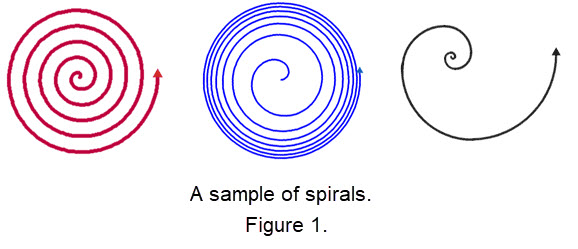
We will focus on spirals on a plane.

There are a variety of spirals. Here is a short list of classic spirals, including their names, equations, and descriptions.

Circle: The trivial spiral, with equation \(r = k\) and comment "The trivial spiral". (The equation is a polar equation.)
The Archimedean spiral: It is also known as the "arithmetic spiral". It is a spiral named after the 3rd-century BC Greek mathematician Archimedes. It is the locus corresponding to the locations over time of a point moving away from a fixed point with a constant speed along a line that rotates with constant angular velocity. Equivalently, in polar coordinates \((r, \theta)\) it can be described by the polar equation \(r = b \cdot \theta\) with real number \(b\).

In polar coordinate form, the equation of the Archimedean spiral below is \(r = \theta\), where \(r\) is the radius of a circle and \(\theta\) is an angle in standard position. For each point graphed on the Archimedean spiral in the polar coordinate plane, the length of any radius of a concentric circle equals the angle measure in standard position.

Several red points are graphed in the polar coordinate plane from 0 to 2\(\pi\) for the Archimedean spiral above. Connecting the points with a "smooth" curve creates a rotation of the spiral.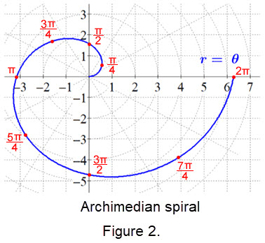
A logarithmic spiral: Such spirals are often called "growth" spirals. It is a self-similar spiral curve that often appears in nature. The first to describe a logarithmic spiral was Albrecht Dürer (1525) who called it an "eternal line" ("ewige Linie"). More than a century later, the curve was discussed by Descartes (1638), and later extensively investigated by Jacob Bernoulli, who called it Spira mirabilis, "the marvelous spiral". In polar coordinates \((r, \phi)\) the logarithmic spiral can be written as \(\boldsymbol{r = ae^{k\phi}}\) with \(e\) being the base of natural logarithms, and \(a \gt 0, k \neq 0\).
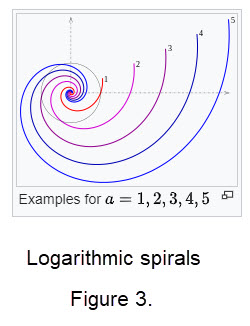
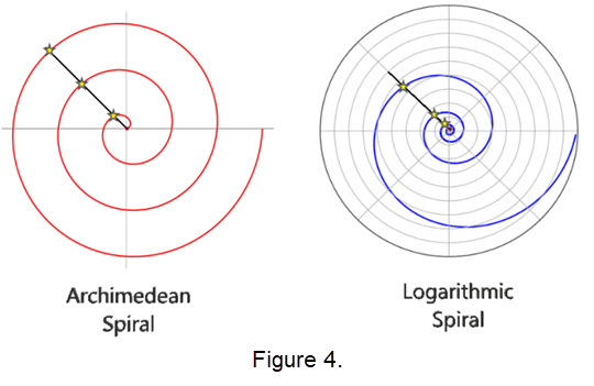
The logarithmic spiral can be distinguished from the Archimedean spiral by the fact that the distances between the turnings of a logarithmic spiral increase in geometric progression, while in an Archimedean spiral these distances are constant. Compare how the placement of the stars vary.
Golden spiral: In geometry, a golden spiral is a logarithmic spiral whose growth factor is \(\phi\), the golden ratio, a ratio between two numbers that which is obtain approximately by the expression \(\mathbf{\phi = \frac{1 + \sqrt 5}{2} \approx 1.618}\). A golden spiral with initial radius 1 is the locus of points of polar coordinates \((r, \phi)\) with polar equation \(\boldsymbol{r = \phi^\frac{2\theta}{\pi}}\). A golden spiral gets wider (or further from its origin) by a factor of \(\phi\) for every quarter turn it makes.
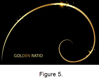
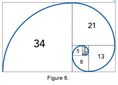
An approximation of the Golden spiral: There are different ways to approximate the Golden spiral. One way is a Fibonacci spiral, which is constructed slightly differently. A Fibonacci spiral starts with a rectangle partitioned into 2 squares. In each step, a square the length of the rectangle's longest side is added to the rectangle. Since the ratio between consecutive Fibonacci numbers approaches the golden ratio as the Fibonacci numbers approach infinity, so does the Fibonacci spiral get more similar to golden spiral the more squares that are added, as illustrated in Figure 6. (A portion of the Fibonacci sequence is 0, 1, 1, 2, 3, 5, 8, 13, 21, 34, 55, 89, 144, 233, 377, 610, 987, 1597, 2584, 4181, … .)

For a view of the Fibonacci spiral that illustrates the squares and the quarter-circle arcs inscribed in squares derived from the Fibonacci sequence click the thumbnail here For a graphical comparison of the golden and Fibonacci spirals click this thumbnail .

Note the symbols that are included.

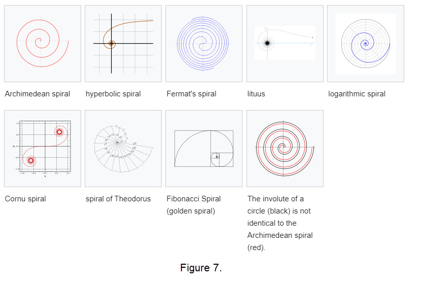
Our list spirals was small to help provide an introduction. Here are examples of some of the most important types of two-dimensional spirals followed by graphs in Figure 7.

The Archimedean spiral \(\mathbf{r = a\theta}\)
The hyperbolic spiral \(\mathbf{r = a/\theta}\)
Fermat's spiral \(\mathbf{a\theta^{1/2}}\)
Euler Spiral: No known Cartesian equation (described as a plane curve)
The lituus \(\mathbf{r = a\theta^{-1/2}}\)
The logarithmic spiral \(\mathbf{r = ae^{k\theta}}\)
The Cornu spiral or clothoid
The Fibonacci spiral and golden spiral
The spiral of Theodorus: an approximation of the Archimedean spiral composed of contiguous right triangles.
The involue of a circle

Note that some spirals, like Fermat's Spiral, Euler Spiral, and Hyperbolic Spiral, do not have known Cartesian equations. These spirals are primarily described in polar coordinates or as plane curves, making it challenging to express them in Cartesian coordinates. The Archimedean spiral is the only spiral with a known Cartesian equation, which is \(\mathbf{x = a\theta}\) and \(\mathbf{y = b\theta}\). The Logarithmic spiral has a Cartesian equation in terms of polar coordinates, but it can be transformed into Cartesian coordinates using trigonometric functions. The remaining spirals lack a known Cartesian equation, and their descriptions are primarily based on their geometric properties or polar coordinate representations. For a longer list of spirals click here More spirals; some with Cartesian equations.

Where are polar curves used?

Polar curves have applications in various fields, including:

Physics and Engineering: To describe the motion of objects in polar coordinates, such as the trajectory of a projectile or the orbit of a celestial body.
Computer Graphics: To create realistic simulations of natural phenomena, like sunsets or aurora, or to design intricate patterns and shapes.
Mathematics: To study geometric transformations, symmetry, and the properties of curves and surfaces.

Can spiral shapes be found in nature, and if so, which ones and why?

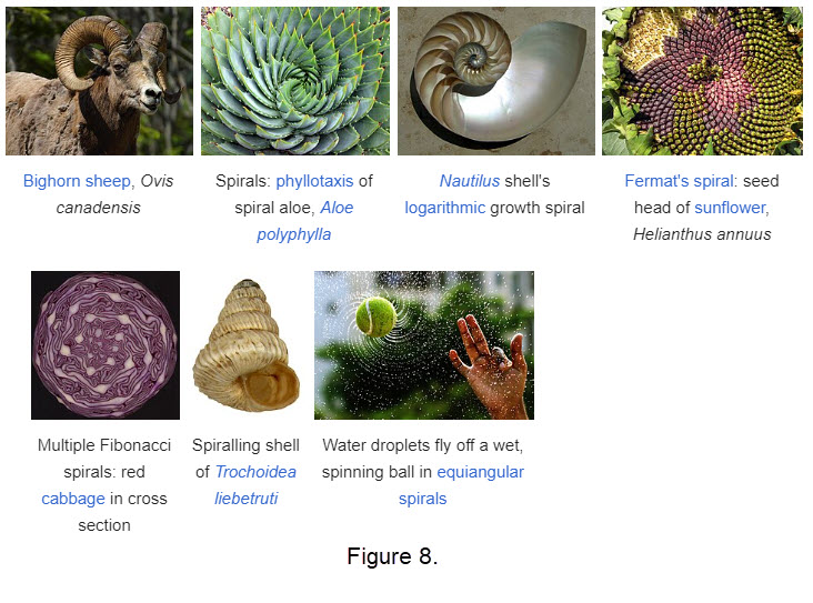
Yes, spiral shapes can be found in nature. According to the search results, spirals appear in various natural phenomena, including:

DNA double helix
Sunflowers
Path of draining water
Weather patterns (including hurricanes)
Vine tendrils
Phyllotaxis (leaf arrangement on plant stems)
Galaxies
Horns of various animals
Mollusk shells
Nautilus shells

These spirals often exhibit self-similarity, meaning they maintain the same shape at different scales. The logarithmic spiral, in particular, is common in nature, as seen in the approach of a hawk to its prey and the approach of an insect to a source of light.

The golden ratio (1.61803) is also closely related to spirals in nature. For example, the nautilus shell is an example of a logarithmic spiral that follows the golden ratio. This ratio is believed to be an efficient and compact way for organisms to grow and develop. The search results also highlight the ubiquity of spirals in nature, from giant galaxies to the smallest gastropod shells.

The presence of spirals in nature may be attributed to their efficiency, predictability, and ability to optimize growth and development.

In summary, spiral shapes are widespread in nature, appearing in various forms and scales, often exhibiting self-similarity and following mathematical patterns like the golden ratio.

The Nautilus shell often enters when spirals are discussed. You can find images of nautilus shells and spirals all over the Internet that are labeled as golden ratios and golden spirals, but this golden spiral constructed from a golden rectangle is nothing at all like the spiral of the nautilus shell, as shown by clicking the thumbnail . This had led many to say that the Nautilus shell has nothing to do with the golden ratio. (Use your browser to find lots of other applications and nature's features.)

==================================================================

SOURCES: The internet contains a large collection of information on spirals. We have tried to present a description of spirals with a review of polar topics. Portions of this work includes descriptions, figures, and thumbnails from a variety of sources. The following list cites items we incorporated that we feel can help students and instructors to learn and enjoy. You can click the links in this list to pursue more information on polar topics.

==================================================================

To draw polar curves:

==================================================================

A few OTHER things:

==================================================================

David R. Hill: click below to see more in mathdemos.org.

Demos for instructors and/or students

The Best of Demos with Positive Impact

An Online Resource for Mathematics Instructors

NEW DEMO

SPIRALS

What is a spiral?