Related Rates

In differential calculus, related rates problems involve finding a rate at which a quantity changes by relating that quantity to other quantities whose rates of change are known. The rate of change is usually with respect to time. Because science and engineering often relate quantities to each other, the methods of related rates have broad applications in these fields. Differentiation with respect to time or one of the other variables requires application of the chain rule, since most problems involve several variables. ( Wikipedia)

Suggested prerequisites: Basic differentiation including the power rule, chain rule, and implicit differentiation. Familiarity with fundamental relationships between components of geometric figures like triangles, circles, rectangles, cones, and spheres.

Many students have difficulty with developing a mathematical model for a related rate problem. Some of the difficulty stems from a lack of geometric visualization skills so that the written description of how things change over time can be translated into an algebraic form. An animation of changes over time can help students focus on salient features of the geometric figure involved and hence provide an opportunity to algebraically relate the changing portions of the figure. With this in mind we have developed a some animations that illustrate a variety of standard related rate situations.

An outline of the general approach to setting up related rate models. The steps list below are really interrelated and are ordered merely as a guide so students have a starting point for aspects of the solution process. The steps involved are illustrated with several examples. We then provide a collection of statements of related rate problems together with visual demos that can be used within a lecture or assigned for students to use for practice. We expect the user is to supply the algebra and calculus to accompany the situation.

Outline of steps in a related rate problem.

1. Recognition: Each related rate problem has a "character" of its own. The diversity of situations to be modeled is an issue that tends to inhibit students from seeing a pattern for the solution process. This is made more abstract by the fact that most related rate problems are posed as (dreaded) word problems. So the algebraic portions of the problem are imbedded within verbal descriptions that connect various components of the problem. Students need some guide posts to assist with recognition other than the fact that the title of the section is Related Rates. Several suggested guide posts that can useful are:
   • Related rate problems often involve a situation in which you are asked to calculate the rate at which one quantity changes with respect to time from the rate at which a second quantity changes with respect to time.
   • Related rate problems can be recognized because the rate of change of one or more quantities with respect to time is given and the rate of change with respect to time of another quantity is required.
   Certainly, the recognition process depends on "reading the problem", which is often given as step 1 in text books.
   
2. Read the problem: The reading of course must be accompanied by understanding. For beginning students one reading is rarely sufficient. The first reading can be used to get familiar with the general situation (the "character") of the problem.
   • Is a geometric figure mentioned?
   • What are the features of the process and/or figure?
   For this reading identification of what is going on at every instant in time is a primary goal. A second (or later) reading can be used to focus on a geometric model of the general situation. Here is where an accompanying animation can provide practice with the visualization of components changing. It is at this point that we usually tell the student to draw a diagram, that is, a geometric embodiment of the process described in the problem statement. This is a key interpretive step, and we need to devise ways for students to practice this step. (See some animations that are included later.)
   
3. Label the diagram: Here the components of the diagram are to be identified as described in the verbal description. It important that the student interpret correctly which parts of the figure are changing with respect to time and any parts that remain fixed throughout. Here again using an animation as part of an example can aid in distinguishing between these two aspects of the problem. Basically, there will be two (or more) varying quantities, but additional information in the problem concerning sizes of quantities at a particular instant of time can lead to difficulty. We must emphasize that no numerical values should be assigned to any quantity varying with respect to time until after the derivative is taken. (See Step 5.)
   
4. Find an equation linking the varying quantities: The result of this step is completely dependent on the "character" of the problem. It is possible that two or more equations must be combined to get a single equation that relates the quantities that vary with respect to time. Certain fundamentals arise repeatedly involving right triangles, rectangles, circles, cones, and spheres.
   
5. Differentiation: Before differentiating, the student should be strongly encouraged to write down the quantity to be determined. Generally this is the rate of change of one of the quantities with respect to time so students should learn that they expect to solve an equation for a derivative expression. Take the derivative implicitly with respect to time of both sides of the equation constructed in Step 4. That is, $$\frac{d}{dt}\Big(\textit{left side}\Big) = \frac{d}{dt}\Big(\textit{right side}\Big)$$ Solve for the rate identified as the one requested in the statement of the problem. Recall that there will be other rates in the expression that result from the implicit differentiation.
   
6. Insert specific information: Substitute specific numerical values for quantities that varied with respect to time and any rate information that was specified. Simplify to obtain a specific expression for the rate requested in the statement of the problem.
   

We present several examples of situations that employ related rates to solve a problem. The way the situation is stated will help set up steps like those suggested above.

Example 1. A spherical balloon is being inflated with a gas at the constant rate of 4 in³/sec . Determine the rate of change of the radius of the sphere. The figure below shows frames from an animation where have we inserted the radii. (The animation can be viewed by clicking the link Inflating a Sphere .)

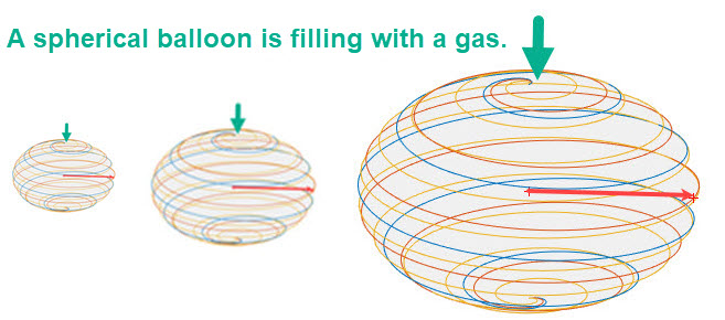
The figure displays that the radius of the sphere changes as the gas is pumped into the sphere. Both the volume and the radius of the sphere change as time goes on. For a formula for connecting these two features, V(t) and r(t), we can use the formula for the volume of a sphere as shown in the following equation:

\[V(t) = \Large \frac{4}{3}\Large \pi \ (r(t))^3 \]

The next step is to differentiate this equation. We must use implicit differentiation with respect to t.

$$\Large\frac{dV}{dt} = \Large\frac{4}{3}\Large \ \pi \ \Large \frac{d(r(t))^3}{dt}$$

The result of the differentiation is \[\Large \frac{dV}{dt} = \Large 4\Large \pi \ \Large(r(t))^2 \ \frac{d(r(t))}{dt}\]

Recall that the spherical balloon is being inflated with a gas at the constant rate of 4 in³/sec so \(\Large \frac{dV}{dt}\) is a constant. Solving for \(\Large \frac{d(r(t))}{dt}\) and simplifying we obtain the rate of change of the radius of the balloon which is $$\Large\frac{d(r(t))}{dt}=\Large \frac{\Large 1 }{\pi r(t)^2} $$

When the radius is 5.5 in then the instantaneous rate of change of the radius is computed as \[\Large r^{'}(t) =\Large \frac{d(r(t))}{dt}=\Large \frac{\Large 1 }{\pi (5.5)^2} = 0.0152 \textit{ in/sec}\]

As the sphere enlarges the rate of change of the radius deceases rather quickly as shown in the table of ordered pairs and the corresponding graph below.

\[ \begin{array}{|c|c|} \hline \bf{Radius} & \mathbf{\Large {\frac{d(r(t))}{dt} }} \\ \hline \text{1} & \text{0.3183} \\ \hline \text{1.5} & \text{0.1415} \\ \hline \text{2} & \text{0.0796} \\ \hline \text{2.5} & \text{0.0509} \\ \hline \text{3} & \text{0.0354} \\ \hline \text{3.5} & \text{0.0260}\\ \hline \end{array} \]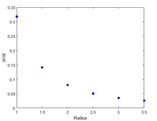

We focused on the radius of the balloon, but a related aspect is its surface area. The surface area, \(\large S(t)\), of a sphere increases quickly as the radius increases and the balloon inflates. The formula for S(t) is

\[\Large S(t) = 4 \ \Large \pi \ \Large (r(t))^2\]

and the formula for the rate of change of the surface area, \(\Large \frac{dS(t)}{dt}\), is

\[\Large \frac{dS(t)}{dt} = 8 \ \Large \pi \ r(t) \Large \frac{dr(t)}{dt}\]

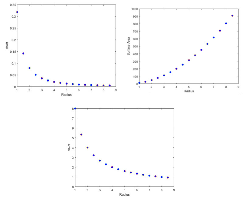
It is instructive to compute the surface area S(t) and the rate of change of S(t) for the balloon.. The surface area increases quickly while its rate of change decreases rapidly. The following sets of ordered pairs indicates this behavior.

\[ \begin{array}{|c|c|} \hline \text{Radius} & S(t) \\ \hline \text{1} & \text{12.5664} \\ \hline \text{1.5} & \text{28.2743} \\ \hline \text{2} & \text{50.2655} \\ \hline \text{2.5} & \text{78.5398} \\ \hline \text{3} & \text{113.0973} \\ \hline \text{3.5} & \text{153.9380}\\ \hline \end{array} \]

\[ \begin{array}{|c|c|} \hline \text{Radius} & \Large {\frac{dS(t)}{dt} } \\ \hline \text{1} & \text{8} \\ \hline \text{1.5} & \text{5.3333} \\ \hline \text{2} & \text{4} \\ \hline \text{2.5} & \text{3.2} \\ \hline \text{3} & \text{2.6667} \\ \hline \text{3.5} & \text{2.2857}\\ \hline \end{array} \]

The accompanying graphs provide a good look at the behaviors for a set of larger radii of the sphere.

Extended look at the sphere balloon problem:

"Mathematics is the study of patterns, both quantitative and spatial. As such, it is the key to understanding our natural and technical world. Through the study of mathematics, students develop skills in problem solving, critical thinking and clear, concise writing." (Just search using a browser using 'mathematics the science or study of patterns' to find books related to the topic and the preceding quote.)

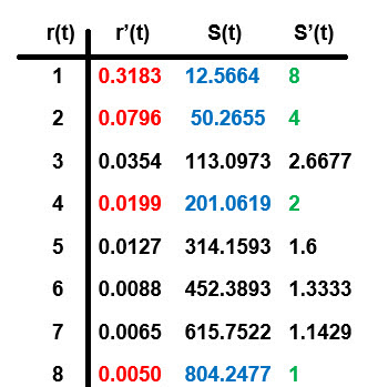
Our related rate example involved inflating a spherical balloon at a fixed rate of 4 in³/sec . Using formulas for the volume and the surface area of a sphere we were able to develop information about rates of change for the radius and the surface area. Let's suppose we put those formulas away and imagine that some 'helpful group' sent us a data table in place of the formulas. (See the data table to the right.) The data table has columns for the radius, r(t), the rate of change, r'(t), the surface area, S(t), and the rate of change of the surface area, S'(t), as the sphere was inflated.

We have an opportunity to use the data table to seek patterns in each of the three columns that contain colored data sets. In each of these three columns the colored entries contain information for values when the radius, r(t), has been doubled. HINT: To help obtain the patterns the value \(\large \pi\) is involved. Since the data table contains only four decimal places, possibly rounded, use your imagination and calculator to help develop the patterns. After you feel you have the patterns formulate an entry for each column for r(t) = 16.

Triangles and Related Rates: The example on the spherical balloon relied on formulas that we could differentiate to obtain rates of change. There are a number of well-known related rate problems that involve creating triangles to aid in developing formulas that can be used to obtain related rates involving time. Many of these problems use geometry to help set up the involved triangles. Here is a short list:

• Airplane and observer.
• Conical tank with a fluid.
• Shadow and a walking person.
• Sliding ladder.
• Conical sand pile.
• Searchlight revolving.
• Baseball diamond with a runner.

The triangles involved in such problems may lead to using similar triangle properties or the Pythagorean Theorem. In either case the differentiation is implicit with respect to time.

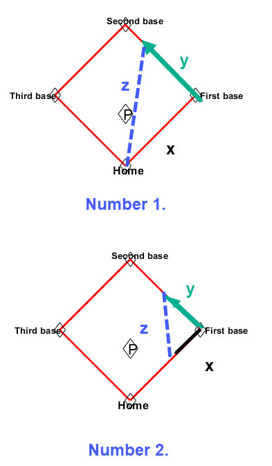
Example 2. Let's consider a baseball diamond with two situations:

1. A runner who is on first tries to steal to get to second base.
2. A runner is on first and a team mate hits the ball past the short stop. The hitter runs to first base while the runner on first heads toward second base.

In each case we can "geometrically" set up a diamond in which a triangle shows the action. (Look at the figure below.) The base paths are each 90 feet and there is right angle at each base.

• Number 1 information: We label the path from home to first by x; as the runner moves toward second suppose that when his rate of speed is \(12 ft/sec\) he is 23 ft from second base; label the distance from first to that point y; label the distance from home to the runner at that time z. We have data enough to find the rate of change of the distance from home to the runner.


• Number 2 information: Suppose the hitter is running toward first at a rate \(15 ft/sec\) when he is 40 feet from first and the runner is moving toward second at the rate of \(18 ft/sec\) when he is 35 feet from second; label the distance the hitter is from first with x; label the distance from first to the runner with y; label the distance from the hitter to the runner by z. We have data enough to find the rate of change of the distance from the hitter to the runner.

The images below illustrate these two scenarios.

Each of the situations outlined above can use the Pythagorean Theorem to obtain the related rate. For a detailed look at a baseball diamond related rate problem click on the following link Baseball Demo. The demo provides a step-by-step solution to a related rate example.

To illustrate several types of related rates click on this link Related Rates Slide Show. It is a slide show that has four examples.

More on Running Bases

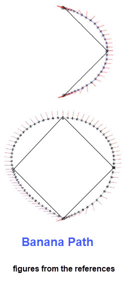
Our related rate problems on runners/hitters running the bases assumed that they would take a straight line between the various bases. This may be correct for stealing a base, but certainly not the case for a hitter who hits the ball to the outfield and expects to get more than a single. In such a case the hitter leaves home at an angle so he can make a quick turn at first by just stepping on a coroner of first base and head towards second base. Such a path is called a " banana path" and depends on the angle used to leave home. If the runner determines to head toward second base there is a similar "banana path". (Look at the figures below.) If the runner continues past second heading to third there is another similar path behavior. As one would expect, a runner that is trying for in the park home run travels again on a "banana path" from third base to home.

Naturally from a mathematical view point the following question arises: What is the optimal path for a base runner? This is interesting since a student at Williams College ask this question and it subsequently led to a published work involving the student and several faculty. There are two good places to read more on this topic; the first is a quick summary and the second is an in depth work that developed a model for the optimal path: Huffpost.com and Optimal Path .

"The model's only assumption is an upper bound on the runner's acceleration vector, which we take to be 10 feet per second per second for the times given here. For a better runner the acceleration might be greater and the times correspondingly faster, but the optimal path is the same. The markings around our optimal paths show the acceleration, forward at the beginning and end, leftward for most of the path." (From the Huffpost.com summary.)

A short variety of related rates.

The related rates technique is an application of the chain rule with first derivatives. Related rates problems can be identified by their request for finding how quickly some quantity is changing when you are given how quickly another variable is changing. It should be used carefully because it does not work with higher order derivatives, or with derivatives of functions of several variables. Here are a few examples.

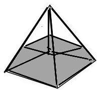
1. Pyramid Tank Problem: In the figure below the base is a square of 10 feet on a side. The vertex is 15 feet and the tank contains a heavy fluid of dept 5 feet. The fluid is pumped into the base at the rate of 4 cubic feet per minute. Find the rate of change of the dept of the fluid in the tank.

   

2. Resistors in Parallel Formula: In electric circuits, it is often possible to replace a group of resistors with a single, equivalent resistor. The equivalent resistance of a number of resistors in parallel can be found using the reciprocal of resistance, \(\large \frac{1}{R}\). The reciprocal of the equivalent resistance is equal to the sum of the reciprocals of each resistance.
   In a circuit two resistors, \(R_1\) and \(R_2\), are connected in parallel. The total resistance \(R\) measured in ohms (denoted by \(\Omega\)) is given by the equation \( R = \large \frac{1}{R_1} + \large \frac{1}{R_2}\). If \(R_1\) is increasing at the rate of \(1.3 \Omega/min\) and \(R_2\) is decreasing at the rate \(0.8 \Omega/min\) at what rate does \(R\) change when \(R_1 = 12 \Omega\) and \(R_2 = 30 \Omega\)?


3. Change in revenue with respect to cost: Consider the cost, \(C\), and revenue, \(R\), information for a type of metal bolt, \(B\) (which represents an inventory of the bolts), given by the formula \(R = 40B - .02*B^2\), and given that \(\large \frac{dC}{dB }= 18\). Find the rate of change of revenue with respect to cost, \(\large \frac{dR}{dC}\), when \(B = 90\). Note: we do not have a formula that lets us solve for revenue as a function of cost.


4. Cobb-Douglas production function reflects the relationships between its inputs - namely physical capital and labor - and the amount of output produced. It's a means for calculating the impact of changes in the inputs, the relevant efficiencies, and the yields of a production activity. Here's the basic form of the Cobb-Douglas production function:" \[Q(L,K)=A*L^\beta*K^\alpha\]
   "In this formula, Q is the quantity produced from the inputs L and K. L is the amount of labor expended, which is typically expressed in hours. K represents the amount of physical capital input, such as the number of hours for a particular machine, operation, or perhaps factory. A, which appears as a lower case b in some versions of this formula, represents the total factor productivity (TFP) that measures the change in output that isn't the result of the inputs. Typically, this change in TFP is the result of an improvement in efficiency or technology. The Greek characters alpha and beta reflect the output elasticity of the inputs. Output elasticity is the change in the output that results from a change in either labor or physical capital."
   
   For example, if the output elasticity for physical capital \(K\) is 0.60 and \(K\) is increased by 20 percent, then output increases by 3 percent (0.6/0.2). The same is true for the output elasticity of labor: an increase of 10 percent in \(L\) with an output elasticity of 0.40 increases the output by 4 percent (0.4/0.1). ( Study.com)
   
   A related rates problem: A toy manufacturer's production function is given by \[Q(L,K)=35*L^{0.40}*K^{0.20}.\] Currently the business uses 12 units of labor and 52 units of physical capital. Assume that the quantity, \(Q\), is a constant, but new technology is available and the board of directors is interested in purchasing it. In addition, assume that both \(L\) and \(K\) are functions of time. Suppose \(\Large \frac{dK}{dt} = 4\), then determine the value of \(\Large \frac{dL}{dt}\). (A calculator is recommended.)