NEW DEMO
Polar Function Gallery
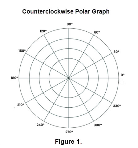
Polar curves are not drawn using the (x, y) coordinates corresponding to horizontal and vertical axes (called Cartesian coordinates). Instead, polar curves are drawn using polar coordinates. The first of the polar coordinates of a point is r: the distance between the point and the pole (the pole is another name for the origin (0, 0), and this distance r is often referred to as the radius). The second of the polar coordinates is \(\mathbf{\theta}\) (read as "theta"): the angle formed by a ray (beginning at the pole extending to the point) and the polar axis (essentially the x-axis). A polar curve is simply the resulting graph of a polar equation which is defined by coordinates \(\mathbf{\text{(r,} \theta)}\). The ordered pairs are graphed on a polar grid as shown in Figure 1.To generate the ordered pairs we use a polar equation \(\mathbf{r = f( \theta)}\) where r is the value of a polar function evaluated at an angle \(\mathbf{\theta}\). (A portion of this introduction appeared in Counting Rose Petals.)
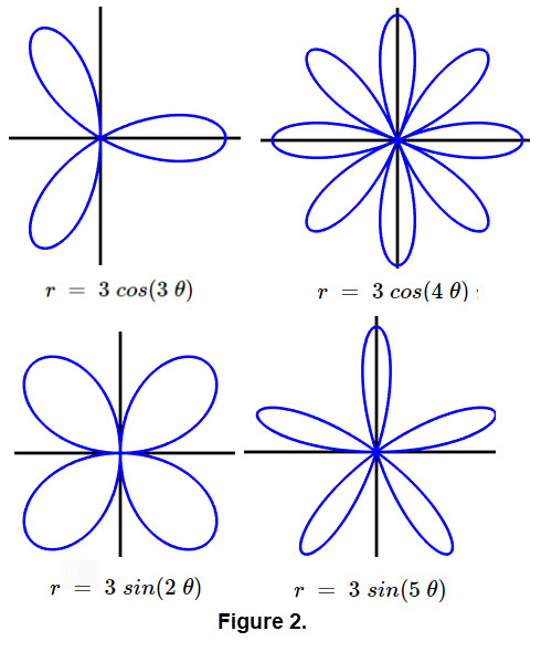
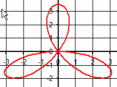
A common type of polar curve is a rose curve which has quite a bit of history. The simplicity and symmetry of Rhodonea or rose curves have fascinated mathematicians since they were first named by the Italian mathematician Guido Grandi in the 1700s. These curves created fascination due to the interesting patterns for the number of petals of the curves. The functions in this case are trigonometric expressions \(\mathbf{ \color{green}{r = } \color{red}{a} \color{green}{*cos(} \color{blue}{b} \color{green}{* \theta)} }\) and \(\mathbf{ \color{green}{r = } \color{red}{a} \color{green}{*sin(} \color{blue}{b} \color{green}{* \theta)}} \). The number of petals that are present will depend on the value of \(\mathbf{ \color{blue}{b}}\). The value of \(\mathbf{\color{red}{a}}\) will determine the length of the petals. There are a wide variety of rose curves. If \(\mathbf{ \color{blue}{b}}\) is an even integer, then the rose will have \(\mathbf{ \color{blue}{2b}}\) petals. If \(\mathbf{ \color{blue}{b}}\) is an odd integer, then the rose will have \(\mathbf{ \color{blue}{b}}\) petals. Several rose curves with a various number of petals appears in Figure 2. The animations for rose curves in the gallery below show how things can change using controls.
Polar Gallery
The following is a gallery
of demos for illustrating selected families of functions. These figures and animations can be used by instructors in a classroom setting or by
students to aid in acquiring a visualization background relating to the change
of parameters in expressions for functions. Two file formats, gif and MP4, are used and should run on most systems. Originally, see the NOTES below the
gallery of animations, the animations were gif files which had no control for a user. The animations are now MP4 files which allow the user to easily control features
like stop and go, restart, and change the animation screen size. The controls are similar to those in You Tube. Click this thumbnail
![]() to see an example.
to see an example.
Gallery of Animations
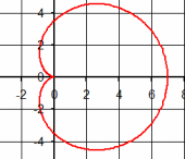
| \(\Large{\text{Cardioids}}\) \(\mathbf{\Large{ \color{green}{r = } \color{red}{a} \color{green}{(1- cos( \theta))} }}\) |
|
Vary a
MP4 Animation Tracing: MP4 Animation |
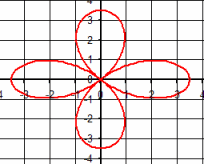
| \(\Large{\text{Rose Curves}}\) \(\mathbf{ \Large{ \color{green}{r = } \color{red}{a} \color{green}{*cos(} \color{blue}{b} \color{green}{* \theta)} }}\) |
|
Vary a
MP4 Animation Vary b MP4 Animation Tracing: MP4 Animation |
| \(\Large{\text{Rose Curves}}\) \(\mathbf{ \Large{ \color{green}{r = } \color{red}{a} \color{green}{*sin(} \color{blue}{b} \color{green}{* \theta)}} }\) |
|
Vary a
MP4 Animation Vary b MP4 Animation Tracing: MP4 Animation |
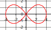
| \(\Large{\text{Lemniscates}}\) \(\mathbf{ \Large{ \color{green}{r^2 =}\color{red}{ a^2}\color{green}{*cos(2\theta)} }}\) |
|
Vary a
MP4 Animation |
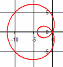
| \(\Large{\text{Limacons}}\) \(\mathbf{ \Large{ \color{green}{r =}\color{red}{a} \color{green}{*cos(\theta) + }\color{blue}{b} } }\) |
|
Vary a
MP4 Animation Vary b MP4 Animation |
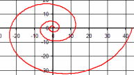
| \(\Large{\text{Equiangular Spiral}}\) \(\mathbf{ \Large{\color{green}{r = e}^{ \color{red}{a} \color{green}{*\theta} } }}\) |
|
Vary a
MP4 Animation |
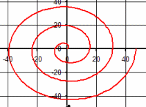
| \(\Large{\text{Spiral of Archimedes}}\) \(\mathbf{ \Large{ \color{green}{r = } \color{red}{a} \color{green}{*\theta} }}\) |
|
Vary a
MP4 Animation |
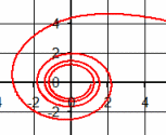
| \(\Large{\text{Lituus}}\) \(\mathbf{ \Large{ \color{green}{r^2 = \frac{\color{red}{a}^2}{\theta}}} }\) |
|
Vary a
MP4 Animation |
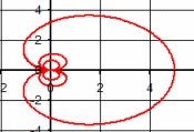
| \(\Large{\text{Cochleoids}}\) \(\mathbf{ \Large{ \color{green}{r =} \frac{\color{red}{a} \color{green}{*sin(\theta)}} {\color{green}{\theta}}}}\) |
|
Vary a
MP4 Animation |
| \(\Large{\text{Conic Sections}}\) \(\mathbf{\Large{ \color{green}{r = } \frac{\color{red}{k} \color{green}{*} \color{blue}{e} } { \color{green}{1 - } \color{blue}{e } \color{green}{* cos(\theta)} }} } \) |

|
Vary k
MP4 Animation Vary e MP4 Animation |
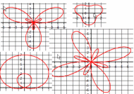
| \(\Large{\text{Rose 'Style' Curves}}\) \( \mathbf{ \Large{\color{green}{r = } \color{red}{c} \color{green}{*} \color{red}{a} \color{green}{* sin(} \color{red}{b} \color{green}{* \theta)} }} \) |
|
Vary ALL of c, a, b
MP4 Animation |
NOTES
- This demo is a modification of a demo in the project Demos with Positive Impact , National Science Foundation's Course, Curriculum, and Laboratory Improvement Program under grant DUE 9952306. managed by David R. Hill and Lila Roberts. The project was based on submitted ideas from instructors. The original demo appeared in 2006.
- Special thanks to Deane Arganbright of University of Tennessee at Martin and to Walter Hunter at Montgomery County Community College for their assistance with the development of the Excel files that were used to get this gallery. The book "Mathematical Modeling with Excel", by Erich Neuwrith and Deane Arganbright (Brooks-Cole) provides a rich source of information for developing Excel routines for mathematical instruction.
- This gallery was developed by David R. Hill, Temple University.
Some Sources for Rose Curves
Other Sources for Polar Curves
- Polar Power: Geogebra applications.
- Some Animations This is a collection of 8 animations of polar curves including spirals, rose curves and limacons. As each curve is generated a table of values is displayed.
- Collection of Polar Curves This is a collection of polar curves which is part of Eric Weisstein's World of Mathematics. Associated with each curve is a wealth of information.
- Another Collection Another collection which has some interesting presentations of polar curves as well as others.
- Plane Curves
- Polar Graphs
- How to Read a Polar Graph