NEW DEMO
Partial Derivatives, Geometrically
The objective of this demo is to provide a visual foundation for partial derivatives of functions of two variables, \(\mathbf {z = f(x,y)}\).
Refresher on first derivatives: To skip this click below.
Derivatives are defined as the varying rate of change of a function with respect to an independent variable.
The derivative is primarily used when there is some varying quantity, and the rate of change is not constant. The derivative is used to measure the sensitivity of one variable (dependent variable) with respect to another variable (independent variable). In a calculus course the topics discussed include what are derivatives, the definition of derivatives, and limits in derivatives in detail.
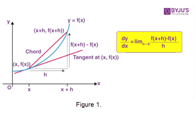
As part of the motivation for the derivative of a function \(\mathbf{y = f(x)}\) of a single variable at a value \(\mathbf{x = a}\), we often draw a set of chords (also called secant lines) which 'settle' into the tangent line position. This provides a visual model for the limit process as illustrated in Figure 1.
|
A first derivative measures the rate of change of a function with respect to one of its variables. It represents the slope of the tangent line to the function's graph at a specific point. In other words, the first derivative describes how the function changes as its input changes, providing an instantaneous rate of change. For more information on limits click here; Limits: via Examples (very little algebra) plus a Calculus example
Symbols and a bit of history.One common symbol for the derivative of a function is Leibniz notation. They are written as the quotient of two differentials \(\mathbf{dy}\) and \(\mathbf{dx}\) which were introduced by Gottfried Wilhelm Leibniz in 1675. It is still commonly used when the equation \(\mathbf{y = f(x)}\) is viewed as a functional relationship between dependent and independent variables. The first derivative is denoted by \(\mathbf{\frac{dy}{dx}}\), read as "the derivative of \(\mathbf{y}\) with respect to \(\mathbf{x}\)". This derivative can alternately be treated as the application of a differential operator to a function \(\mathbf{\frac{dy}{dx} = \frac{d}{dx} f(x)}\) or \(\mathbf{f'(x)}\).
Referring to Figure 1, if we let the value of \(\mathbf{x}\) change along the curve \(\mathbf{y = f(x)}\) we can see that the tangent lines change slope. The values of the slopes generate the derivative
function, which is denoted \(\mathbf{f'(x)}\). We can think of the function \(\mathbf{f '(x)}\) as having its values generated by the slopes of the moving tangent line segments as shown in the following animation.
Click this thumbnail
![]() to see the animation.
to see the animation.
Applications
- Optimization: First derivatives are used to find the maximum or minimum of a function.
- Physics: First derivatives describe the motion of objects, including velocity and acceleration.
- Economics: First derivatives are used to model the behavior of economic systems and optimize functions.
By understanding the properties and rules of first derivatives, you can analyze and model various phenomena in mathematics, physics, economics, and other fields.
Note: Portions of the preceding discussion are from Derivatives, Wikipedia Derivatives, and an AI search using the browser BRAVE. An another good refresher and list of derivative rules is at Calculus introduction.
===============================================================================
Partial Derivatives
In mathematics, a partial derivative of a function of several variables is its derivative with respect to one of those variables, while holding all the others constant. This concept is essential in analyzing surfaces for maximum and minimum points and gives rise to partial differential equations.
Think of a function as a surface in 3D space. When you take a slice of the surface using a plane parallel to one of the axes (for example, the x-axis), you get a 2D function. The partial derivative represents the rate of change of the function along that slice, with the other variables (y, z, etc.) held constant.
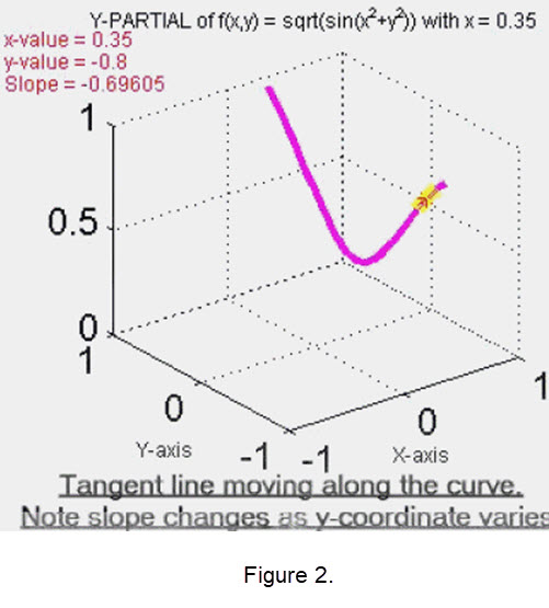
The description of the first derivative is applied when we want to discuss the 'partial' derivatives of \(\mathbf{z = f(x,y)}\) with respect to \(\mathbf{x}\) or \(\mathbf{y}\). For instance, one of the unknowns is held fixed at a particular value say, \(\mathbf{x = 0.35}\). See Figure 2. We then take a plane perpendicular to the x-axis at this location and slice the surface to generate a curve which has equation \(\mathbf{z = f(0.35, y)}\). Then the partial derivative of \(\mathbf{f}\) with respect to \(\mathbf{y}\) when \(\mathbf{x = 0.35}\) corresponds to the slope of a tangent line moving along this curve. In this case since \(\mathbf{x}\) is fixed the values of the slopes of the tangent lines trace out produce a partial derivative in \(\mathbf{y}\).
|
To see the an animation that contains Figure 2, click this thumbnail
![]()
Common notations for partial derivatives for \(\mathbf{z = f(x, y)}\) include:
- \(\mathbf{f_x}\) or \(\mathbf{\frac{\partial{f}}{\partial{x}}}\) for the partial derivative with respect to \(\mathbf{x}\)
- \(\mathbf{f_y}\) or \(\mathbf{\frac{\partial{f}}{\partial{y}}}\) for the partial derivative with respect to \(\mathbf{y}\)
Suppose, we have a function \(\mathbf{f(x, y)}\), which depends on two variables \(\mathbf{x}\) and \(\mathbf{y}\), where \(\mathbf{x}\) and \(\mathbf{y}\) are independent of each other. Then we say that the function \(\mathbf{f}\) partially depends on \(\mathbf{x}\) and \(\mathbf{y}\). Now, if we calculate the derivative of \(\mathbf{f}\), then that derivative is known as the partial derivative of \(\mathbf{f}\). If we differentiate the function \(\mathbf{f}\) with respect to \(\mathbf{x}\), then take \(\mathbf{y}\) as a constant and if we differentiate \(\mathbf{f}\) with respect to \(\mathbf{y}\), then take \(\mathbf{x}\) as a constant.
Note: Portions of the preceding discussion are from Wiki Partial derivatives and Byjus Partial derivatives. The Byjus link discusses the limits used in partial derivatives and provides worked examples.
Computing partial derivatives step-by-step for \(\mathbf{z = f(x, y)}\).
- Step 1: Identify the variable with respect to which we have to find the partial derivative.
- Step 2: Except for the variable found in Step 1, treat all the other variables as constants.
- Step 3: Differentiate the function just using the rules of ordinary differentiation.
Wait! Read Step 3 again. Yes, the rules of ordinary differentiation apply to partial differentiation. In partial differentiation, just treating variables is different, that's it! For more details click here Cuemath
Partial Derivative Gallery
The following is a gallery
of demos for illustrating selected 3D surfaces. These animations can be used by instructors in a classroom setting or by
students to aid in acquiring a visualization background relating to the change
of parameters in expressions for partial derivatives. The file formats are MP4 which should run on most systems. Originally, see the NOTES below the
gallery of partial derivatives, the animations were gif files which had no control for a user. The animations are now MP4 files which allow the user to easily control features
like stop and go, restart, and change the animation screen size. The controls are similar to those in You Tube. Click this thumbnail
![]() to see an example.
to see an example.
| \(\large{\text{Surface}}\) | \(\large{\text{Picture}}\) | \(\large{\text{Click the}}\) \(\large{\text{animation}}\) |
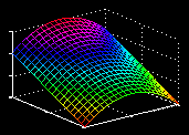
| \(\large{z = f(x, y) = x^2 + y}\) \(\large{y-partial}\) |
|
==>
MP4 Animation |
| \(\large{z = f(x, y) = x^2 + y}\) \(\large{x-partial}\) |

|
==>
MP4 Animation |
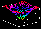
| \(\large{z = f(x, y)}\) \(\large{= \sqrt{sin(x^2 + y^2)}}\) \(\large{y-partial}\) |
|
==>
MP4 Animation |
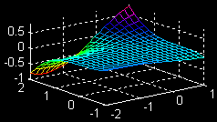
| \(\large{z = f(x, y)}\) \(\large{=\frac{1}{9} y^3 sin(x)}\) \(\large{x-partial}\) |
|
==>
MP4 Animation |
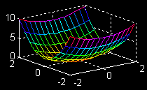
| \(\large{z = f(x, y)}\) \(\large{= 0.5x^2+ 2y^2}\) \(\large{x-partial}\) |
|
==>
MP4 Animation |
| \(\large{z = f(x, y)}\) \(\large{= 0.5x^2+ 2y^2}\) \(\large{y-partial}\) |

|
==>
MP4 Animation |
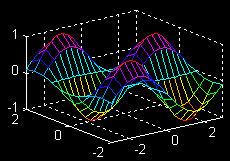
| \(\large{z = f(x, y)}\) \(\large{= sin(x)cos(2y)}\) \(\large{x-partial}\) |
|
==>
MP4 Animation |
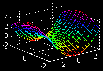
| \(\large{z = f(x, y)}\) \(\large{= 0.5x^2 - 0.5y^2}\) \(\large{x-partial}\) |
|
==>
MP4 Animation |
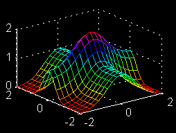
| \(\large{z = f(x, y)}\) \(\large{= e^{-x^2} + e^{-4y^2} }\) \(\large{y-partial}\) |
|
==>
MP4 Animation |
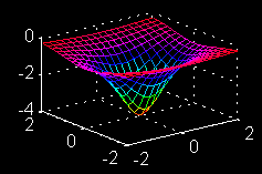
| \(\large{z = f(x, y)}\) \(\Large{= \frac{-4}{1 + x^2 + 2y^2} }\) \(\large{x-partial}\) |
| ==>
MP4 Animation |
NOTES
- This demo is a modification of a demo in the project Demos with Positive Impact , National Science Foundation's Course, Curriculum, and Laboratory Improvement Program under grant DUE 9952306. managed by David R. Hill and Lila Roberts. The project was based on submitted ideas from instructors. The original demo appeared in 2006.
- Surfaces and animations generated in MATLAB.
- This gallery was developed by David R. Hill, Temple University.
==================================================================
For more calculus demos in mathdemos.org click below.