NEW DEMO

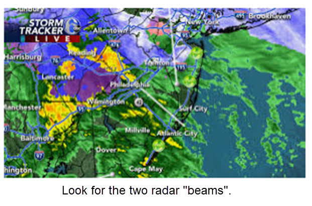
"In earlier times, before the telegraph and the telephone were invented, weather observations from faraway places could not be collected in one place soon after they were made. In those times, the only way of predicting the weather was to use your local experience. Given the weather on a particular day, what kind of weather usually follows during the next day or two? As you can imagine, the success of such forecasting was not a lot better than making a random guess." For a bit more history click here Weather history. It was widely thought that things were like the contents of the following gif.

The development of radar significantly changed our ability to improve forecasting. "The concept of RAdio Detection and Ranging (Radar began in the late 1800's and by World War II, radar was in use by militaries around the world, scanning for incoming airplanes. But the use of radar for weather observations occurred by accident. Analysts noted in periods of heavy weather, the radar would return strange signals. Investigation into this phenomenon resulted in the discovery that these echoes were returns from the precipitation, unmasking a further use for the technology. In 1942, the U.S. Navy donated 25 surplus radars to the National Weather Service (then known as the Weather Bureau), marking the start of a U.S. weather radar system. The technology was refined and in 1959 the NWS began rolling out its first network of radars dedicated to a national warning network. An updated version, the WSR-74, supplemented and replaced the older radars beginning in 1977. These radars provided similar data but with newer and more reliable components." Click here Weather and radar to see where this paragraph came from and further information about Doppler radar.

Radar systems transmit electromagnetic, or radio, waves. Most objects reflect radio waves, which can be detected by the radar system. The frequency of the radio waves used depends on the radar application. Weather radar (also known as Doppler weather radar) is an instrument that sends pulses of electromagnetic energy into the atmosphere to find precipitation, determine its motion and intensity, and identify the precipitation type such as rain, snow or hail. It is not unrealistic to think that the radar signals can be viewed as random tools to gather data that can then be used in computer forecasting models to predict future weather trends, while alerting meteorologists to upcoming precipitation, storms or severe weather. Thus radar provides a way decipher how far away precipitation is, its speed and how big are droplets or snowflakes. Radar is a technique that uses simulation which is a way of collecting probability data using actual objects like radio waves. With this point of view radar is a type of Monte Carlo simulation which is discussed next.

The objective of this demo is to illustrate the relationship between probability and the approximation of the area of a region in the Cartesian plane (a two-dimensional coordinate plane, which is formed by the intersection of the x-axis and y-axis). This is an introduction to topics which include introductory probability, simulation topics, and numerical approximation. Our primary tool is the technique known as Monte Carlo simulation which provides an approach to estimate probabilities. In mathematics, the theory of random (also called stochastic) processes is an important contribution to probability theory.

For an example consider coin tossing. It is well known that to approximate the probability of obtaining a head in coin tossing, we may toss the coin repeatedly, counting the number of heads obtained, and then divide that number by the total number of tosses. This simple idea has extensions to more complex experiments. For a specified event, perform the experiment repeatedly, count the number of favorable outcomes, and then divide that number by the total number of times you perform the experiment. We would like to use this basic idea to determine the relationship between probability and area by performing a sequence of simulations.

The term "Monte Carlo Method" is very general. A Monte Carlo method is a technique, that is based on using random numbers and probability to investigate problems. Monte Carlo methods are employed in a wide variety of fields including economics, finance, physics, chemistry, engineering, and even the study of traffic flows. Each field using Monte Carlo methods may apply them in different ways, but in essence they are using random numbers to examine some problem and approximate its outcome. As such Monte Carlo methods give us a way to model complex systems that are often extremely hard to investigate with other types of techniques.

Here is a bit of history: "The term 'Monte Carlo' was introduced by von Neumann and Ulam during World War II, as a code word for the secret work at Los Alamos; it was suggested by the gambling casinos at the city of Monte Carlo in Monaco. The Monte Carlo method was then applied to problems related to the atomic bomb." ( Simulation and the Monte Carlo Method by Reuven Y. Rubinstein, John Wiley & Sons, Inc., New York, 1981, p.11.) For a more on the history of Monte Carlo methods click here Monte Carlo history.

We have four Cartesian colored figures within a black box in Figure 1. You can approximate the area of these figures using simulations. We want to use a number of simulations to construct a sequence of approximations that hopefully will provide information in the form of a probability that we can accept and leads to an area computation of the colored figure in Figure 1. This a task that will require patience and careful examination of the set of approximations.

To illustrate the Monte Carlo method we randomly select and plot points in the 8 by 8 black square. Each of the colored figures will have some points that have the corresponding color. When you use the program below you will be able to display a number of points in a simulation by clicking the button again. The black square and the colored figure within will begin to fill with points. .This simulates steps of the Monte Carlo method. Click a simulation's button several times to see the action of increasing the total number of points used. For an example, click the following thumbnail images.

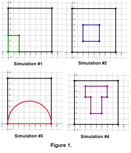
To experiment with the Monte Carlo method on the simulations shown in Figure 1 click Execute RANDOM plots on a SIMULATION. We suggest that you experiment with each of the simulations to try to observe the rate at which the points are filling areas.

The Monte Carlo method for this demo uses 2 BIG STEPS plus other needed support features.

• #1 Estimate the probability of a dot "falling" in a colored figure.


• #2 Estimate the area of the colored figure.


• For each simulation we can get an estimated probability by computing the ratio of the number of dots in the colored figure divided by the total number of dots used. The hard part is to obtain a good estimate of the probability. To do this we usually need to obtain a set of estimates of the probability and then use that data to determine a value of the probability to use in the area estimate.


• The area estimate is easy: AREA ESTIMATE of a colored figure = probability times the area of the "black box". Certainly from the grids in Figure 1 we know that the black box has an area of 64 square units.

The following program can be used to perform a series of experiments. It focuses on estimating the probability of a dot falling in the colored figure. Carefully follow the directions in the fall-down windows that appear and other directions that are shown on the screen. Click on Estimate the Probability of a SIMULATION. There is a "checker" that can give information about the accuracy of the estimated probability of a dot falling in the colored figure. Do several simulations on the same figure that appears in Figure 1 and record the probability in each case. Then try to estimate a value of the probability to use in the area estimate. You can do the math to estimate the area of the colored figure.

The probability can vary quite a bit depending on the total number of ordered pairs used in the simulation. Hopefully using experiments with an increasing number of dots we can generate a sequence of approximate probabilities that seem to be converging to a specific value. Suggestion: try using a small number of dots then rerunning the experiment with a larger number of dots. There can be surprises.

In Figure 2 we have an example of a set of approximate probabilities for a simulation of a figure in a box similar those in Figure 1. It took a number of trials to collect this data. You will notice that probabilities for a selected number of ordered pairs can vary quite a bit. Also note that there are instances where the probability estimate for a small number of ordered pairs is close to a probability that used a large number of ordered pair. The analysis of such data to determine a good estimate of the probability of a dot falling in the colored figure inside the black box is difficult. The term data mining is used in a situation like this. "Data mining is the process of searching and analyzing a large batch of raw data in order to identify patterns and extract useful information." For more information click on the following source More on Data Mining.

OPTIONAL/OPPORTUNITY

Note that in Figure 2 some estimates are missing. Your job is to use the program below to supply an estimate of the missing data. You can try to estimate for a missing spot several times if you want to. Once you are satisfied with the whole set of data try to estimate a good probability based on the data. That is, play being a "Data Miner". ( WARNING: choose the correct number of dots used for those missing in Figure 2. You can take a screen picture of Figure 2 to print out and to use as you fill the missing datum.)

The following program can be used to perform a series of experiments. Carefully follow the directions in the fall-down windows that appear and other directions that are shown on the screen. Click on Estimate the Probability for Data Mining. There is a "checker" that can give information about the accuracy of the estimated probability of a dot falling in the colored figure.

WHAT MATH IS USED ?

The simulations are based on using randomly generated ordered pairs. There are several features in our programs that we want to elaborate.

• How do we generate ordered pairs for the dots?
  
  In the computer programs that are available there is a built in feature that lets the user generate random numbers. We used the following javascriipt commands.
  function generateRandomFloatInRange(min, max) { return (Math.random() * (max - min )) + min;}
  We called the function twice, one for an x-value and another for a y-value. There are other variations to include the min and max values and to obtain integers. For convenience items in Figure 1 used the first quadrant of the Cartesian grid. We set our min = 0 and max = 8 to limit things in the black box. This code can be used to aid in obtaining figures that are in other quadrants. Click the following thumbnail to see an example.


• How did we get dots in the colored figures?
  
  An ordered pair for a dot it is guaranteed to "fall" in the black box using the "function" above, but we need to test to see if it would "fall" in the colored figure. If it did "fall" in the colored figure we would use the corresponding color instead of black to display the dot. Suppose the situation is that the ordered pair (xpt, ypt) is guaranteed to fall in the black box. But we want to see if it would "fall" in a rectangular colored figure which has the dimensions described as, horizontally from A to B (along the x-axis) and vertically from C to D (along the y-axis). If it did not fall in the colored rectangle it was a black dot elsewhere in the black box.
  
  Using the code below in Figure 3 determine how to replace the question marks (??) with the letters the, A, B, C and D that describe the smaller rectangle.

  

  For example let A = -2, B = 3, C = -4, D = 2 be the data for a small rectangle within a larger rectangle. Assume that dot (-3, 0) would fall in the big rectangle, but will it fall in the colored small rectangle? Use the code in Figure 3. How about dot (1,1)? Don't cheat by using the geometric image for the rectangles.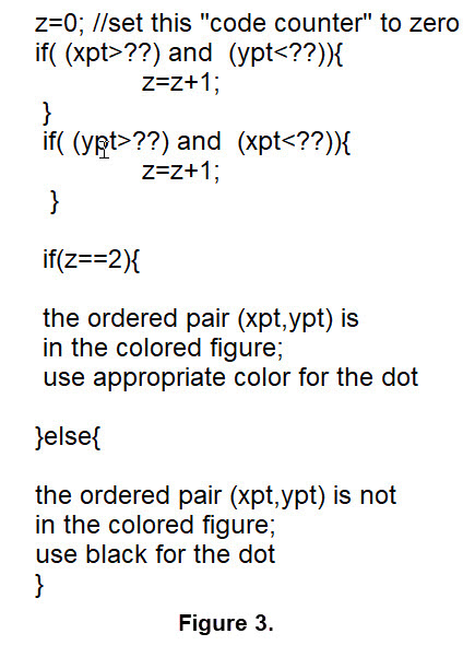
  
  
• For #3 Simulation in Figure 1 we need a different approach to determine if an ordered pair is in the semi circle. HINT: use the radius of the semi circle and a distance formula.
  
  
• For #4 Simulation in Figure 1 conjecture how we were able to get the two different colored dots in the "T" figure. Click the thumbnail to see simulation for this situation.
• If you took the opportunity for the data mining example you saw a figure like the thumbnail . How do you determine when a dot falls in the triangle? HINT: Using the coordinates of the dot and those of the triangle you can build 3 other triangles. If the sum of the areas of the 3 triangles is less than the area of the original triangle the dot is in inside the original triangle. The key is how do you compute the areas of the triangles. Click on Area of a Triangle. and investigate the content.

Area under a Curve

Another type of problem involves an algebraic function f(x) in which a portion of its graph is in a rectangular box. In this case we will want to estimate of the area under the curve. For example, click on the thumbnail shown here . This type of figure is often met in calculus where you employ integration of f(x) over a specified interval along the x-axis. Similar techniques are used to obtain an acceptable value of the probability of a dot falling in the blue figure here as those used previously. Carefully follow the directions in the fall-down windows that appear and other directions that are shown on the screen. Click on Estimate the AREA under the Curve. There is a "checker" that can give information about the accuracy of the estimated probability of a dot falling in the colored figure. For this problem you should obtain a set of estimates for the area under the curve then determine what seems to be acceptable. You can check that value in the checker. Don't be surprised how often you need to use the simulations in this approach. Also note that the number of dots used is chosen randomly in this routine. (Have fun!)

This approach to estimate the area under the curve is known as a Monte Carlo integrator. It can also be used to approximate volumes under surfaces in higher dimensions. In fact this technique was used at Los Alamos during the very early days of computing to solve some very difficult differential equations in higher dimensions.

Other Information and Related Material

• Try to derive an equation for the function in the area under the curve example and compute the area. Hint: use sin(x), cos(x), and the constant 3.


• Suppose the ordered pair (x,y) is in the simulation of 'dots' for the area under the curve routine. What selection of x or y would guarantee that the dot is not in the blue figure?


• For those who want a detailed foundation for the Monte Carlo integrator, click on the thumbnail which contains a development using expected value.

Thanks

Portions of this demo are based on the work created by Dr. Anthony Berard (retired), Department of Mathematics, King's College (Pennsylvania). We thank him for permitting us to use certain materials. His work was originally included in Demos with Positive Impact, A Project to Connect Mathematics Instructors with Effective Teaching Tools, which was supported by a grant from the National Science Foundation's Course, Curriculum, and Laboratory Improvement Program: DUE-9952306.