New Demo

A common game at carnivals and fund raisers involves COIN TOSSING. There are various forms of such games. Click the thumbnail to see a hand carved coin toss "board". It is hard to see but the small holes in this board are different sizes since coins may have a different diameter like modern "change". Such boards make it difficult to determine information how to toss winners. (A carnival board is usually much larger than this antique.)

The game we investigate in this demo consists of a board with a grid of uniform squares as shown in Figure 1. The objective of the game is toss a coin onto the board. If the coin lands entirely within a square then you win a prize, otherwise you lose your coin. In Figure 1 the red circles indicate winners.

To see a Coin Toss Simulation click on this thumbnail . You may notice that the toss of a coin onto the board often does not fully lie in a square. We will use two different boards, one 4 by 4 and the other 5 by 5. The size of the board may play a role in accumulating circles that fall completely inside a square. To get a feel for simulating a coin toss game by tossing a variety of the number of coins, we suggest you try both of the following activities.

There are two activities, one on a 4 by 4 board and another on a 5 by 5 board. On each board the squares are 100 by 100 units, the circles have a radius of 30 units, and the user can click a button to add 5 more circles to the board. The button can be clicked as many times as you like and you can click another button to restart the activity. The math used behind the scene is to randomly generate ordered pairs (x, y) that fall within the board and then draw the circle using (x, y) as its center. The key to determine whether a circle falls completely within a square is checked using that the length of the radius from the center must stay within the sides of the square to be a winner.

TWO ACTIVITIES: Try both several times.

• For the 4 by 4 board the random ordered pair (x, y) uses values from 1 to 400. To use this activity click here Tosses on a 4 by 4 board.
  
  
• For the 5 by 5 board the random ordered pair (x, y) uses values from 1 to 500. To use this activity click here Tosses on a 5 by 5 board.

To see how to compare the two activities we experimented by counting the number of winners (red circles) when we used 500 coins with a radius of 20 units to toss 10 times on each activity. The results are shown in Figure 2.

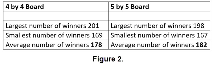
This small data set doesn't prove anything, but certainly indicates that the number of squares in boards of this type, squares of 100 by 100 units, may not influence the number of winners when the same size coin is used. We invite you to try a similar experiment with a radius of 25 or 30 to see if pattern results are similar to that shown in Figure 2.

Finding MATH for our Coin Tossing

A primary objective of this demo is to illustrate the use of statistical simulation to find a rule which will lead to the prediction of probabilities. There are a variety of places where this demo can be used including, general math classes in high school or college, elementary probability courses, or probability courses for math majors. Prerequisites involve basic probability concepts and properties of circles and squares. Any computing environment, which supports random number generation including calculators can be used, but here we use java script. (Our two activities are in java script.)

A player soon realizes that the chances of winning are related to the size of the squares and the size of coin used. So the design of the board and the type of coin used are important to entice players to participate, yet have the game operator not give away too many prizes. Determining the design of the game can be investigated in two ways:

• Fix the diameter of the coin, but vary the size of the squares.
  
  
• Fix the size of squares but vary the diameter of the coin.
  
  

In our development we will fix the size of squares and vary the diameter of the coin. Since countries have different sizes of coins for various monetary denominations we employ rather generic dimensions. The discussion can be specialized for various sizes of coins. We present two approaches. Approach 1 uses a game based approach of tossing experiments to get an idea of the approximate probability of a winning toss. Approach 2 concentrates on finding a formula for estimating the probability of a winning toss by a simple construction.

Approach 1. Suppose a single square on the board has dimensions s x s, while the coin has radius r so its diameter d = 2r. The crucial question is: What constraint should be imposed on the location of the center of the circle to be declared a winning toss?

Certainly we know that if d is less than s and if the center of the coin coincides with the center of the circle we have a winner. Imagine now we that have a single square board (made on paper) of size s x s and a coin (made of paper) with d is less than s. Put a pin in the center of the paper coin and move it around the paper board in such a way that we have a winner for each move. For each move use the pin to put a hole in the (paper) board. Assume we do this quite a few times and then look at the pattern of holes.

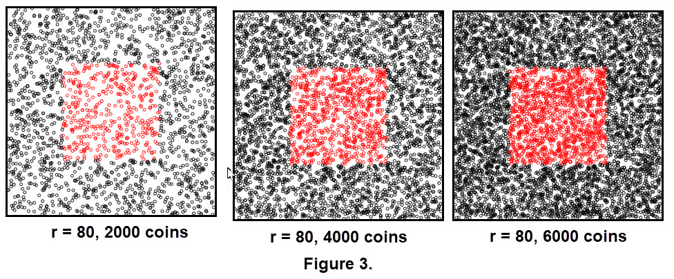
We have constructed a single square with s = 300 units. Next we tossed lots coins on the square and recorded the centers of the circles (and deleted showing the circles). The red dots are centers of circles which are "winners" and black dots are "looser's". Examine Figure 3, where we used r = 80 units and show the pattern of the winners vs. looser's.

We chose the larger single square to be able to see how images of the red dots changed. To see a corresponding figure for a single 100 by 100 square click on the thumbnail . This image is basically a compression of Figure 3, note the value of r used.

As the number of coins increases the red figure takes on the shape of a square in both single squares. If we used say, 8000 or more coins, the denser the red figure becomes.

We simulated the coin toss game using s = 300 with r = 80 and using s = 100 with r = 26.66 (about 80/3) for various numbers of tosses. (Some in Figure 3 and the thumbnail.) One way to approximate the probability of a winning toss is to compute the ratio of the number of winners to the total number of tosses used to obtain the dots used for the centers. This procedure is called a Monte Carlo simulation.

Here is a brief explanation of the Monte Carlo Method and how it works.

• The Monte Carlo Method is a computerized mathematical technique that allows people to quantitatively account for risk in forecasting and decision-making. At its core, the Monte Carlo Method is a way to use random samples of parameters to explore the behavior of a complex system. (In our case the parameters involve ordered pairs.)
• Simulate processes that are time consuming.
• Run a large number of experiments in a short time-frame.
• Quickly adjust and repeat experiments.

Next we present a table of such data in Figure 4. Recall that we are using random selection of order pairs for the centers so the ratio is an estimation. (We recorded ratios to 4 decimal places.)

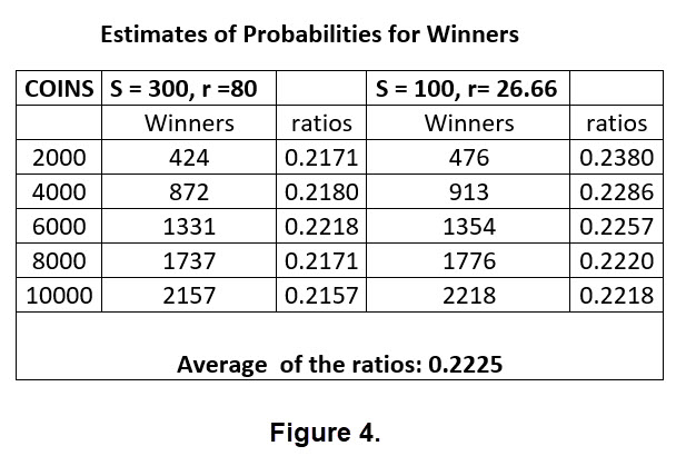
The data seems to imply that the two variations sited above for the choices in s yield very similar results. It also appears that red figure in both choices is a good approximation of a square. If we change the radius for each value of s similar behavior should result.

For another application of Monte Carlo click on Segments and Circles within Circles.

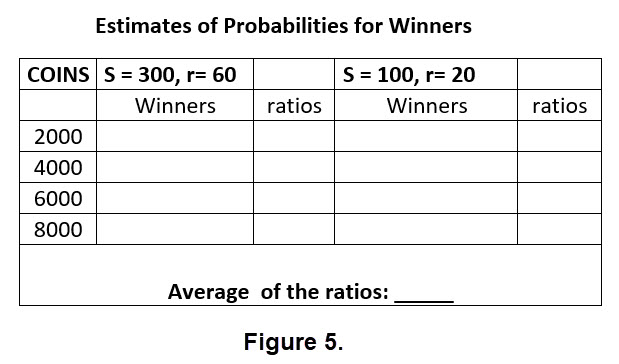
We have activities for estimating the probabilities for both squares 300 by 300 and 100 by 100 which can be used with various radius selections. For instance you might consider r in the 300 by 300 square for values like 40, 60, 80, 120 etc. and change these values appropriately for the 100 by 100 square. Certainly you can experiment with other values.

More Activities:

• For the 300 by 300 square the random ordered pair (x, y) for the center of the circles uses radius values from 30 to 120. To use this activity click here Radius for 300 by 300 square.
  
  
• For the 100 by 100 square the random ordered pair (x, y) for the center of the circles uses radius values from 10 to 40. To use this activity click here Radius for 100 by 100 square.

As an example, fill in the empty areas in Figure 5. Use the results to estimate the probability of a winner for the choice of the radius.

Approach 2. Here we take a close look at a pattern of images like those in Figure 3. We will use the 300 by 300 square to provide a set of images for a variety of choices for the radius of the coin. To illustrate a pattern we will put vertical lines on the single square and suggest an algebraic expression for estimating the probability of a winner.

In Figure 6 we have images that use 50,000 tosses for coins with a different radius for the coins. In each image we super imposed vertical grid lines that should help establish a pattern that appears on all images regardless of the radius. The grid lines are made in a convenient manner for the 300 by 300 single square.

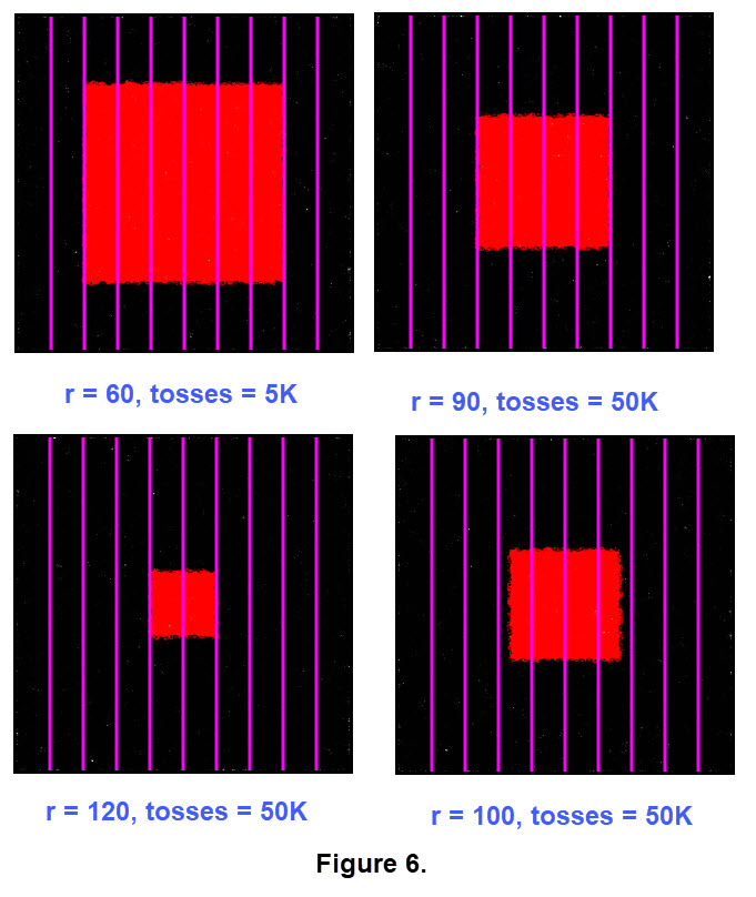
Look at the images in Figure 6. As an aid to help identify a pattern click this thumbnail . Now make a conjecture regarding a pattern in the images in Figure 6.

If you haven't found a pattern that depends on the information in the labels for the images in Figure 6, click this thumbnail .

Next we want to suggest a way to use the pattern to approximate the probability of a winner in the coin toss. The expression \(\large{F(s,r)=\frac{(s-2*r)^2}{s^2}} \) is considered a way to approximate the probability of a winner. Recall that s = 300 is the size of single square and r is the radius of the coin used in a toss. Look at the thumbnail immediately above. If we were ask to consider our images in Figure 6 as just one square inside another square, then we can compute the percentage of the area of the inner square within the larger square by the same formula. (For information of about approximating the area of a figure imbedded in a larger figure, click on AREA via Monte Carlo.) However, we are not using areas here but we can estimate the probability of a winner in a coin toss using the ratio \(\large{R\text{(red dots/total tosses)}= {\frac{\text {number of red dots}}{\text{total number of tosses}}}} \) and then compare it with the output of \(\large{F(s,r)}\).

Next consider Figure 7 which contains a table of simulations and compares our functions\(\large{R}\) and \(\large{F}\). In this table the single square has s equal to 300, each simulation uses 50K tosses, uses the result of the number of red dots, and a few values for the radius r for the coin. The corresponding values of \(\large{F(300,r)}\) are needed for comparison . Fill in the missing values of the table.

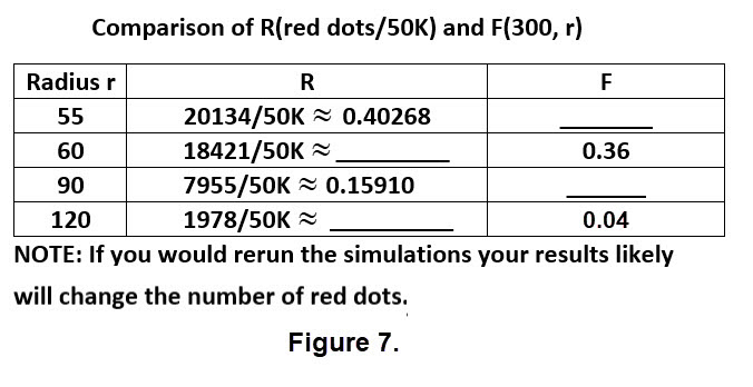
After you have filled in the missing information in Figure 7, what is your opinion of using \(\large{F(s,r)=\frac{(s-2*r)^2}{s^2}} \) to approximate the probability of tossing a winner for the coin toss, at least for the items in Figure 7?

Recall that we made a special board, namely that all squares on the board are the same size. So don't think you can use items like we presented here the next time you participate in a coin toss in the real world. The "house" usually wins!

Math for a Comparison

First, lets simplify \(\Large{\frac{(s-2*r)^2}{s^2}} \). Using algebra we can obtain an equivalent expression that is a quadratic polynomial; let s = 300 and we get \(\large{F(300,r) = \frac{4}{300} r^2 - \frac{4}{300} r + 1}\). The following table shows 10 choices of the radius with computations for 50K simulations, and results of \(\large{F(300,r) }\).

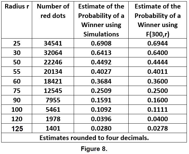
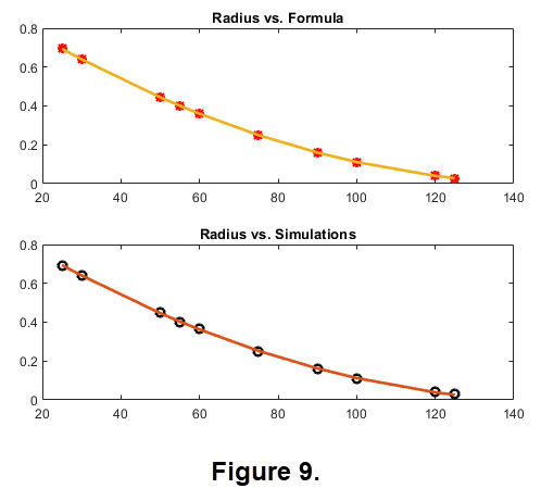
The two estimates of the probabilities in Figure 8 are very close. There is another mathematical procedure we can do to further indicate that these estimates are close for other choices of a radius. We have a quadratic polynomial for \(\Large{F(300,r)}\). To further compare the two estimates we can develop another quadratic polynomial using the radii and the estimates from the simulations. Lets call the estimates in simulation column in Figure 8 sim(k) for k = 1 to 10 and the radii rad(k). We proceed by using the data pairs (rad(k), sim(k)) to generate a least squares quadratic polynomial that gives us an approximate formula to predict probability values for any radius from 25 to 125. First express \(\Large{F(300,r)}\) in decimal form: \(\Large{0.4444*10^{-4}r^2 - 0.1333*10^{-1}r +1}\). We computed the least squares quadratic polynomial \(\Large{P(r) = 0.4295*10^{-4}r^2 - 0.1313*10^{-1}r + 0.9947}\). (Both quadratics are rounded to 4 decimal places.)

The final step is to graph the two quadratics. Figure 9 shows the graph of each quadratic. If they were super imposed they would appear with only a small variation.

A least squares quadratic polynomial (also called quadratic regression) is the process of finding the equation of the parabola that best fits a set of data. As a result, we get an equation of the form \( y=ax^2+bx+c\) where coefficient a is not equal to 0. The term best fits means we are required to minimize an error term that involves the vertical distance from a data pair to the curve. For further information click here Least Squares Quadratic Curve Fitting. NOTE: The quadratic least squares for the radii and simulations appears to have the ordered pairs on the curve. In many cases the ordered pairs may be near the graph or even quite a bit away from it. Click here to see an example. The topic of least squares appear in a variety of STEM areas; in math courses it appears in statistics, numerical analysis, and linear algebra.

Other Resources

• As a web exercise, have students search for coin toss games similar to that described here that have a different configuration to the board or some other way for players to win.
  
  
• M. Haruta, MFlaherty, J. McGiveney, and R. McGiveney, "Coin Tossing", Mathematics Teacher, Vol. 89, No. 8, November 1996, p. 642-645.
  
  
• A Matlab program, which can be downloaded and copied by clicking Matlab demo, functions differently than the activities in this demo. The images of the circles representing the coin tosses are retained with winners appearing in red. The radius can be any value in the interval (0,4.9). To see an animation of this program click here Toss Simulation.
  
  
• For other probability demos click on mathdemos.org and look in the topics Geometry and More.

Acknowledgment

Portions of this demo are based on the work originally created by Demos with Positive Impact, A Project to Connect Mathematics Instructors with Effective Teaching Tools, which was supported by a grant from the National Science Foundation's Course, Curriculum, and Laboratory Improvement Program: DUE-9952306.